4.35. Viscoplastic-viscoSCRAM Model

4.35.1. Theory

The viscoSCRAM model is an isotropic, linear viscoelasticity model with isotropic damage for modeling particulate composite materials. The bulk material is treated as viscoelastic while damage is governed by a statistical crack mechanics (SCRAM) theory [[1]] which accounts for material damage from the nucleation and growth of microcracks. Damage can occur from bond breakage within the binder, between the binder and particulates, and within the particulates. The crack growth kinetics assume non-interacting cracks and include no mechanisms for shear dilation such as from particulate debonding and rotation. The viscoSCRAM model captures linear viscoelastic shear rate-dependence and inelastic deformation associated with damage. The viscoSCRAM model is based on the papers by Hackett and Bennett [[2]] and Buechler and Luscher [[3]] with a modified implementation.

The viscoplastic-viscoSCRAM model [[4]] is an extension of the viscoSCRAM model to include pressure-dependent viscoplasticity and volumetric dilation. The linear viscoelasticity and damage mechanics of the viscoSCRAM model remain largely unaltered, but are embedded within a yield surface plasticity model. Prior to plasticity, the model reduces identically to the viscoSCRAM model. The viscoplastic-viscoSCRAM model draws on elements of the papers by Buechler [[5], [6]] as well as standard viscoplasticity theory from Kojic and Bathe [[7]].

The deviatoric strain \(e_{ij}\) is additively decomposed into a viscoelastic component \(e_{ij}^{ve}\), a damage component \(e_{ij}^D\), and a viscoplastic component \(e_{ij}^p\) as

(4.178)\[e_{ij} = (e_{ij}^{ve} + e_{ij}^{D}) + e_{ij}^p .\]

The deviatoric stress \(s_{ij}\) depends only on the viscoelastic strain through a generalized Maxwell model as

(4.179)\[\dot{s}_{ij} = 2 G^{\infty} \dot{e}_{ij}^{ve} + \sum_{\kappa=1}^{N} \left( 2 G^{(\kappa)} \dot{e}_{ij}^{ve} - \frac{s_{ij}^{(\kappa)}}{\tau^{(\kappa)}} \right)\]

where \(G^{\infty}\) is the steady-state (rubbery) shear modulus and \(G^{(\kappa)}, s_{ij}^{(\kappa)}, \tau^{(\kappa)}\) are the shear modulus, deviatoric stress, and relaxation time for the \(\kappa^\text{th}\) Maxwell element.

The damage strain is given by

(4.180)\[e_{ij}^{D} = \frac{1}{2 G_0} \left( \frac{c}{a} \right)^3 s_{ij}\]

where \(G_0 = G^{\infty} + \sum_{\kappa=1}^N G^{(\kappa)}\) is the instantaneous shear modulus, \(c\) is the damage parameter representing an averaged microcrack size, and \(a\) is a crack normalizing factor.

The damage parameter \(c\) captures crack growth. It is based on brittle fracture mechanics including stable and unstable crack growth regions. The crack growth rate is

(4.181)\[\begin{split}\dot{c} = \begin{cases} v_{res} \left( \frac{K_I}{K_1} \right)^m & \text{for } K_I < K' \\ v_{res} \left[ 1 - \left( \frac{K_{0\mu}}{K_I} \right)^2 \right] & \text{otherwise} \end{cases}\end{split}\]

where \(v_{res} = min\{v_c\bar{\dot{\varepsilon}}^{v_a} 10^{v_b}, v_{max}\}\) is an empirical relation for the crack speed with fitting parameters \(v_a\) and \(v_b\) and limited by the Raleigh wave speed \(v_{max}\). The coefficient \(v_c\) is included for ease of unit conversion. Here, \(\bar{\dot{\varepsilon}} = \sqrt{\frac{2}{3} \dot{\varepsilon}_{ij} \dot{\varepsilon}_{ij}}\) is the effective strain rate. The exponent \(m\) is a model parameter controlling the shape of the crack growth rate curve. The stress intensity is

(4.182)\[K_I = \bar{\sigma} \sqrt{\pi c}\]

where the effective stress \(\bar{\sigma}\) is computed as

(4.183)\[\begin{split}\bar{\sigma} = \begin{cases} \left( \frac{3}{2} s_{ij} s_{ij} \right)^{\frac{1}{2}} & \text{for } \sigma_m < 0 \\ \left( \frac{3}{2} \sigma_{ij} \sigma_{ij} \right)^{\frac{1}{2}} & \text{otherwise} \end{cases}\end{split}\]

and \(\sigma_m = \sigma_{kk}/3\) is the mean stress. The transition stress intensity \(K'\), marking the boundary between stable (slow) crack growth and unstable (rapid) crack growth, is given by

(4.184)\[K' = K_{0\mu} \left( 1 + \frac{2}{m} \right)^{\frac{1}{2}}\]

where \(K_{0\mu}\) is the frictional threshold stress intensity. \(K_{0\mu}\) reflects the frictional resistance to crack growth under compressive loading which inhibits damage evolution. This tensile/compressive frictional asymmetry is given by

(4.185)\[K_{0\mu} = K_0 \left[ 1 + \frac{\pi \mu' \langle p \rangle \sqrt{c}}{K_0} \left( 1 + \frac{\mu' \langle p \rangle \sqrt{c}}{K_0} \right) \right]^{\frac{1}{2}}\]

where \(K_0\) is the frictionless threshold stress intensity, a model fitting parameter, \(\mu'\) is the friction coefficient, and \(p = -\sigma_m\) is the pressure. Here, \(\langle \cdot \rangle\) are Macaulay brackets.

Finally, the normalizing stress intensity \(K_1\) is defined as

(4.186)\[K_1 = K' \left( 1 + \frac{m}{2} \right)^{\frac{1}{m}} .\]

The damage parameter \(c\) captures crack growth; however, it is not normalized like a traditional continuum mechanics damage parameter. An alternative damage parameter, \(D\), may be defined as

(4.187)\[D = \frac{\left( \frac{c}{a} \right)^3 }{1 + \left( \frac{c}{a} \right)^3},\]

which is 0 for the undamaged state \(c=0\) and asymptotes to 1 for a fully damaged state.

In the viscoSCRAM model, there is no viscoplasticity; that is, the viscoplastic strain component \(e_{ij}^{p} = 0\) in (4.178). For the viscoplastic-viscoSCRAM model, a viscoplastic constitutive response extends the viscoSCRAM model.

The viscoplastic model is based on an overstress assumption; that is, in stress space, the stress point may lie outside the yield surface and move towards the yield surface with time. Viscoplastic flow occurs until the stress point lies on the yield surface. Let \(f(\sigma_{ij},\varepsilon_{ij}^{p},D)\) be the yield surface such that the yield condition is

(4.188)\[f(\sigma_{ij},\varepsilon_{ij}^{p},D) = 0 .\]

The total viscoplastic strain rate is prescribed by a Perzyna model as

(4.189)\[\dot{\varepsilon}_{ij}^{p} = \dot{\lambda} \frac{\partial g}{\partial \sigma_{ij}},\]

with

(4.190)\[\dot{\lambda} = \gamma \langle \phi[f] \rangle,\]

where \(g(\sigma_{ij},\varepsilon_{ij}^{p},D)\) is the flow surface, which is, in general, non-associative. Here \(\gamma\) is a fluidity parameter and \(\phi\) is a functional of the yield surface. The rate of plastic flow is controlled by \(\dot{\lambda}\) while the direction of plastic flow is normal to the flow surface.

For particulate composite materials, common choices for the yield surface \(f\) and flow surface \(g\) are Drucker-Prager forms with potentially different fitting constants. However, the theory is general and allows for any form of yield or flow surface to be prescribed based on the experimental data.

The implemented Drucker-Prager forms for the yield surface and flow surface are defined, respectively, as

(4.191)\[f(\sigma_{ij}) = \sigma_e + A \cdot \sigma_m - \sigma_y \qquad \text{and} \qquad g(\sigma_{ij}) = \sigma_e + B \cdot \sigma_m - \sigma_y ,\]

where \(\sigma_e\) is the equivalent stress given by

\[\sigma_e = \sqrt{\frac{3}{2} s_{ij} s_{ij}},\]

\(\sigma_m\) is the mean stress, \(\sigma_y\) is the yield stress, and \(A\) and \(B\) are fitting constants.

The flow rule is selected to be,

(4.192)\[\dot{\lambda} = \frac{1}{\tilde{\tau}} \langle \frac{f(\sigma_{ij})}{\sigma_0} \rangle^{\tilde{m}},\]

where \(\tilde{\tau}\) is the viscoplastic relaxation time, \(\sigma_0\) is a normalizing constant, and \(\tilde{m}\) is a fitting exponent.

4.35.1.1. Time-Temperature Superposition Principle

The preceding theory embeds the standard mechanical viscoSCRAM theory. The temperature dependent response of viscoelastic materials was not discussed; however, the theory may be extended. The thermo-viscoelastic behavior of a polymer is related to the molecular rearrangement of the material under loading; the speed of this rearrangement is controlled by the temperature [[8]]. For the class of thermorheologically simple materials, one dominant molecular transition controls the response. For these materials, the time-temperature superposition principle is valid. This principle holds that long time relaxation behavior at low temperatures is equivalent to short term relaxation behavior at high temperatures. This manifests as a simple horizontal time shift of the relaxation modulus curve with temperature change.

The generalized Maxwell model (4.179) may be written equivalently in integral form as

(4.193)\[s_{ij} = \int_{-\infty}^{t} 2 G(t-r) \frac{de_{ij}^{ve}}{dr} dr ,\]

where \(G(t-r) = G^{\infty} + \sum_{\kappa=1}^{N} G^{(\kappa)} e^{\frac{-(t-r)}{\tau^{(\kappa)}}}\) is the relaxation spectra. At a reference temperature \(T_{ref}\), the relaxation spectra in terms of logarithmic time is \(G(t-r, T_{ref}) = \hat{G}(log_{10}(t-r))\). For a thermorheologically simple material, time-temperature superposition states that the relaxation spectra at any other temperature \(T\) is a horizontal translation of the reference relaxation spectra; that is, \(G(t-r, T) = \hat{G}(log_{10}(t-r) - log_{10}(a_T(T)))\) where \(a_T(T)\) is the shifting factor. The deviatoric stress at any temperature is then equal to the deviatoric stress at the reference temperature, but at a scaled time; namely, \(s_{ij}(t,T) = s_{ij}(\frac{t}{a_T},T_{ref})\). Reverting to the differential form, the deviatoric stress equation is

(4.194)\[\dot{s}_{ij} = 2 G^{\infty} \dot{e}_{ij}^{ve} + \sum_{\kappa=1}^{N} \left( 2 G^{(\kappa)} \dot{e}_{ij}^{ve} - \frac{s_{ij}^{(\kappa)}}{\tau^{(\kappa)}} \right) ,\]

where the relaxation times are \(\tau^{(\kappa)} = a_T(T) \, \tau^{(\kappa)}_{ref}\) with \(\tau^{(\kappa)}_{ref}\) being the relaxation times at the reference temperature.

The generalized Maxwell equations for the standard mechanical model (4.179) have identical form and are recovered by setting the shift factor \(a_T(T) = 1\). The crack growth kinetics are assumed to be unaffected by temperature, so both formulations use the same implementation with temperature dependence introduced solely through the shift factor.

The shift factor model is defaulted to none (\(a_T = 1\)). Available shift factor models are the Williams-Landel-Ferry (WLF) model, the Arrhenius model, and a user defined model. In these models, the shift factors are defined as

(4.195)\[\begin{split}\textrm{WLF:} \quad log_{10}(a_T) &= \frac{-C_1 \, (T-T_{ref})}{C_2 + (T-T_{ref})}, \\ \textrm{ARRHENIUS:} \quad log_{10}(a_T) &= \frac{E_a}{R} (log_{10}e) \left( \frac{1}{T} - \frac{1}{T_{ref}} \right), \\ \textrm{USER DEFINED:} \qquad \quad \, \, \, \, \,\,\, a_T &= a^{ud}(T) .\end{split}\]

Here, \(C_1\) and \(C_2\) are fitting constants for the WLF model. For the Arrhenius model, \(E_a\) is the activation energy and \(R\) is the gas constant.

Note, time-temperature superposition is verified for the viscoSCRAM component of the model with no viscoplasticity. Time-temperature superposition will run with the full viscoplastic-viscoSCRAM model; however, the theoretical basis with viscoplasticity is still under investigation.

4.35.2. Implementation

The viscoplastic-viscoSCRAM model discretization uses a staggered solution scheme. The damage model has both stable and unstable crack growth branches which causes implicit numerical solution schemes to be highly sensitive, unstable, or difficult to converge. For this reason, the time integration of the deviatoric stress is explicit in the damage variable and implicit in the viscoplastic strain. The solution scheme is staggered between the damage update and viscoplastic update; that is, the damage state variable and Maxwell stresses are held fixed at their converged values from the previous timestep, the viscoplastic strain is updated within a solution loop, and finally, the damage state variable and Maxwell stresses are updated with the new viscoplastic strain held fixed.

The viscoSCRAM component is evaluated with an explicit time integration scheme. Substituting the time derivatives of (4.178) and (4.180) into (4.179), the deviatoric strain rate becomes

(4.196)\[\dot{s}_{ij} = \psi(c) (\dot{e}_{ij} - \dot{e}_{ij}^p) - \theta(c,\dot{c}) s_{ij} - \lambda_{ij}(c,s_{ij}^{(\kappa)})\]

where

(4.197)\[\psi(c) = \frac{2 G_0}{1 + (\frac{c}{a})^3} = 2 G_0 (1-D)\]

and

(4.198)\[\theta(c,\dot{c}) = \frac{3 (\frac{c}{a})^2 \frac{\dot{c}}{a}} {1 + (\frac{c}{a})^3} = \frac{\dot{D}}{1-D}=\]

and

(4.199)\[\lambda_{ij}(c,s_{ij}^{(\kappa)}) = \frac{\sum_{\kappa=1}^{N} \frac{s_{ij}^{(\kappa)}}{\tau^{(\kappa)}}}{1 + (\frac{c}{a})^3} = (1-D) \sum_{\kappa=1}^{N} \frac{s_{ij}^{(\kappa)}}{\tau^{(\kappa)}} .\]

Integrating (4.196) explicitly, the deviatoric stress update becomes

(4.200)\[(s_{ij})_{n+1} = (s_{ij})_{n} + \frac{\Delta t}{(1+\frac{\Delta t}{2} \theta_n) } \left[ \psi_n ((\dot{e}_{ij})_n - (\dot{e}_{ij}^p)_n) - \theta_n (s_{ij})_n - (\lambda_{ij})_n \right] .\]

The mean crack size is updated according to

(4.201)\[c_{n+1} = c_n + \dot{c}_n \Delta t .\]

The Maxwell stress rates can be written in the form

(4.202)\[\dot{s}_{ij}^{(\kappa)} = 2 G^{(\kappa)} (\dot{e}_{ij} - \dot{e}_{ij}^p ) - \frac{s_{ij}^{(\kappa)}}{\tau^{(\kappa)}} - \frac{G^{(\kappa)}}{G_0} \left[ \frac{3}{a} \left( \frac{c}{a} \right)^2 \dot{c} s_{ij} + \left( \frac{c}{a} \right)^3 \dot{s}_{ij} \right]\]

which, when treated as a first-order, linear, constant-coefficient ODE in \(s_{ij}^{(\kappa)}\), may be solved to provide the Maxwell stress update as

(4.203)\[\begin{split}(s_{ij}^{(\kappa)})_{n+1} = (s_{ij}^{(\kappa)})_{n} e^{\frac{-\Delta t}{\tau^{(\kappa)}}} + \\ \left( 1 - e^{\frac{-\Delta t}{\tau^{(\kappa)}}} \right) \left( 2 G^{(\kappa)} \tau^{(\kappa)} ((\dot{e}_{ij})_{n+1} - (\dot{e}_{ij})_{n+1}^p ) - \frac{G^{(\kappa)}}{G_0} \tau^{(\kappa)} \left[ \left( \frac{3}{a}\right) \left( \frac{c_{n+1}}{a}\right)^2 \dot{c}_n (s_{ij})_{n+1} + \left( \frac{c_{n+1}}{a}\right)^3 (\dot{s}_{ij})_{n} \right] \right) .\end{split}\]

Here, the relaxation times are \(\tau^{(\kappa)} = a_T(T_{n+1}) \tau^{(\kappa)}_{ref}\). These times are updated at the start of the time step by computing the shift factor at the new temperature \(T_{n+1}\) and then shifting the reference relaxation times.

The mean stress is updated as

(4.204)\[ (\sigma_m)_{n+1} = (\sigma_m)_{n} + K ((\dot{e}_{ii})_{n+1} - (\dot{e}_{ii})_{n+1}^p) \Delta t\]

and finally the Cauchy stress is updated as

(4.205)\[(\sigma_{ij})_{n+1} = (s_{ij})_{n+1} + (\sigma_m)_{n+1} \delta_{ij} .\]

For the viscoSCRAM model, there is no viscoplasticity (\(\Delta \varepsilon_{ij}^p = \Delta e_{ij}^p = 0\)); both the deviatoric stress update (4.200) and the mean stress update (4.204) are explicit. For the viscoplastic-viscoSCRAM model, both the deviatoric stress update and the mean stress update are implicit in the plastic strain increment.

The viscoplastic flow rate (4.189) is integrated implicitly as

(4.206)\[\Delta \varepsilon_{ij}^p = \Delta \lambda \left( \frac{\partial g}{\partial \sigma_{ij}}\right)_{n+1} ,\]

where the viscoplastic flow increment is

(4.207)\[\Delta \lambda = \gamma \langle \phi[f_{n+1}] \rangle \Delta t .\]

The deviatoric viscoplastic flow rate is the projection

(4.208)\[\Delta e_{ij}^p = \Delta \lambda \left[ \left( \frac{\partial g}{\partial \sigma_{ij}}\right)_{n+1} - \frac{1}{3} \left( \frac{\partial g}{\partial \sigma_{kk}}\right)_{n+1} \delta_{ij} \right] .\]

Defining a trial stress as

(4.209)\[(\sigma_{ij})_{n+1}^{TR} = (s_{ij})_{n} + \frac{\Delta t}{(1+\frac{\Delta t}{2} \theta_n) } \left[ \psi_n (\dot{e}_{ij})_n - \theta_n (s_{ij})_n - (\lambda_{ij})_n \right] + [(\sigma_m)_{n} + K (\dot{e}_{ii})_{n+1} \Delta t] \delta_{ij} ,\]

the Cauchy stress update is then

(4.210)\[(\sigma_{ij})_{n+1} = (\sigma_{ij})_{n+1}^{TR} - \Delta \lambda \left[ \left( \frac{\psi_n}{(1+\frac{\Delta t}{2} \theta_n) } \right) \left( \frac{\partial g}{\partial \sigma_{ij}}\right)_{n+1} + \left( K - \frac{\psi_n}{3(1+\frac{\Delta t}{2} \theta_n)} \right) \left( \frac{\partial g}{\partial \sigma_{kk}}\right)_{n+1} \delta_{ij} \right] .\]

The total stress update (4.210), solved in conjunction with the viscoplastic flow update (4.207), provides seven equations in the seven unknowns \(\{ (\sigma_{ij})_{n+1}, \Delta \lambda \}\). This system of equations is solved with a Newton-Raphson scheme as part of a return map algorithm.

The time integration solution scheme outlined is implicit in the viscoplastic update. For the Perzyna model, this implicit integration is unconditionally stable [[9]]. However, the time integration is explicit for the viscoSCRAM damage update. If the critical timestep is determined by the viscoplastic update, the unconditionally stable implicit integrator is advantageous. If the critical timestep is determined by the damage update, the additional cost of the implicit viscoplastic update is unnecessary and an explicit viscoplastic time integrator may be used. An explicit viscoplastic time integrator is included as an option.

4.35.3. Verification

The viscoplastic and viscoSCRAM responses of the model are verified independently of each other. Coupled, even simple boundary-value problems do not have analytical solutions for the viscoplastic-viscoSCRAM model, nor is code-to-code verification available. However, given the staggered solution scheme implemented, the viscoplastic response is updated holding fixed the viscoSCRAM response and vice versa. For this scheme, independent verification of the individual responses is sufficient. The viscoSCRAM component is verified for a purely viscoelastic response, for the crack growth kinetics from a spherical loading, and for uniaxial compression. The viscoplastic component of the model is verified for uniaxial tension and simple shear.

4.35.3.1. Viscoelasticity

Standard mechanical model The viscoSCRAM component combines standard viscoelasticity with a crack growth damage parameter \(c\). Zeroing the initial crack size, \(c=0\), reduces the model to a viscoelastic model. The crack growth kinetic parameters do not matter in this case. Two Maxwell elements are used for the verification test and the material parameters used are shown in Table 4.58.

Table 4.58 The material properties for the viscoSCRAM model testing viscoelastic response.

\(K\)	5.0 MPa
\(G^{\infty}\)	1.0 MPa
\(c\)	0.0 mm
\(a\)	1.0 mm
\(K_0\)	0.03 MPa \(\sqrt{\textrm{mm}}\)
\(\mu'\)	1.16
\(m\)	10.0
\(v_{max}\)	3.0e5 mm/s
\(v_{a}\)	0.892
\(v_{b}\)	2.28
\(N\)	2
\(G^{(\kappa)}\) (MPa)	1.0	2.5
\(\tau^{(\kappa)_{ref}} (s)\)	1.0	10.0
SHIFT FACTOR MODEL	NONE

A unit cube is fixed in the normal directions on the sides orthogonal to the \(x_3\)-axis and on the bottom in the \(x_3\)-direction. A constant logarithmic strain rate ramp load followed by a holding period is applied to the top of the cube in the \(x_3\)-direction by specifying the applied displacement field as

(4.211)\[\begin{split}u_i = \begin{cases} (e^{\dot{\epsilon} t} -1) X_3 \delta_{i3} & \text{for } t < t_L \\ (e^{\dot{\epsilon} t_L} -1) X_3 \delta_{i3} & \text{otherwise} \end{cases}\end{split}\]

where \(\dot{\epsilon}\) is the strain rate and \(t_L\) is the ramp loading time. Here \(\dot{\epsilon} = 1\) s\(^{-1}\) and \(t_L = 1\) s which corresponds to a \(100\%\) logarithmic axial strain. The logarithmic deviatoric strain rate during loading is

(4.212)\[\dot{e}_{ij} = \frac{1}{3} \dot{\epsilon} (3 \delta_{i3} \delta_{j3} - \delta_{ij}) .\]

The analytical Cauchy stress to this boundary-value problem is then

(4.213)\[\begin{split}\sigma_{ij} = K \dot{\epsilon} t \delta_{ij} - K \dot{\epsilon} (t - t_L) \mathcal{H} (t-t_L) \delta_{ij} + 2 G^{\infty} t \dot{e}_{ij} - 2 G^{\infty} (t - t_L) \mathcal{H} (t-t_L) \dot{e}_{ij} + \\ \sum_{\kappa = 1}^N 2 G^{(\kappa)} \tau^{(\kappa)} (1-e^{\frac{-t}{\tau^{(\kappa)}}}) \dot{e}_{ij} - \sum_{\kappa = 1}^N 2 G^{(\kappa)} \tau^{(\kappa)} (1-e^{\frac{-(t-t_L)}{\tau^{(\kappa)}}}) \mathcal{H} (t-t_L) \dot{e}_{ij}\end{split}\]

where \(\mathcal{H}\) is the Heaviside function.

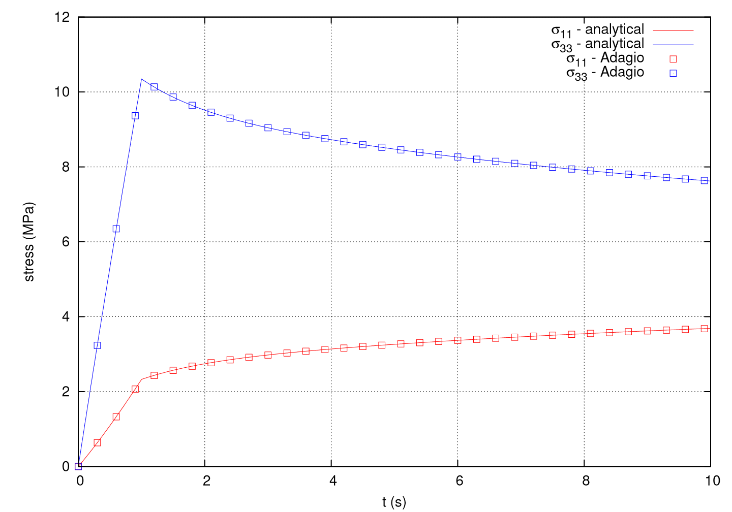
Fig. 4.148 The axial and lateral stresses.

The results of the analysis are shown in Fig. 4.148.

The axial stress \(\sigma_{33}\) increases nearly linearly until the end of the ramp loading, \(t_L = 1\) s, and then relaxes as the displacement is held fixed. Similarly, the stresses \(\sigma_{11} = \sigma_{22}\) increase linearly during ramp loading and then continue to increase as the axial stress relaxes. The Adagio solution shows agreement with the analytical solutions.

Time-Temperature Superposition

The temperature dependence of the viscoelastic model, via the time-temperature superposition principle, is verified for the same boundary-value problem, viscoelastic parameters, and crack growth kinetic parameters. Only the shift factor model is modified. Here, all three shift factor models are verified for isothermal loading. WLF parameters were selected and then Arrhenius parameters calculated to provide an identical shift factor. The user defined function was defined as the WLF equation. The shift factor model parameters used for the verification test are shown in Table 4.59. The isothermal temperature was set to 305 K.

The results of the analysis are shown in Fig. 4.149.

The axial stress \(\sigma_{33}\) increases nearly linearly until the end of the ramp loading, \(t_L = 1\) s, and then relaxes as the displacement is held fixed. Similarly, the stresses \(\sigma_{11} = \sigma_{22}\) increase linearly during ramp loading and then continue to increase as the axial stress relaxes. The Adagio solution shows agreement with the analytical solutions.

Table 4.59 The shift factor model properties for the viscoSCRAM model testing viscoelastic response.

SHIFT FACTOR MODEL	WLF
\(C_1\)	17.44
\(C_2\)	51.6 K
\(T_{ref}\)	300 K
SHIFT FACTOR MODEL	ARRHENIUS
\(E_a/R\)	6.4918e4 K
\(T_{ref}\)	300 K

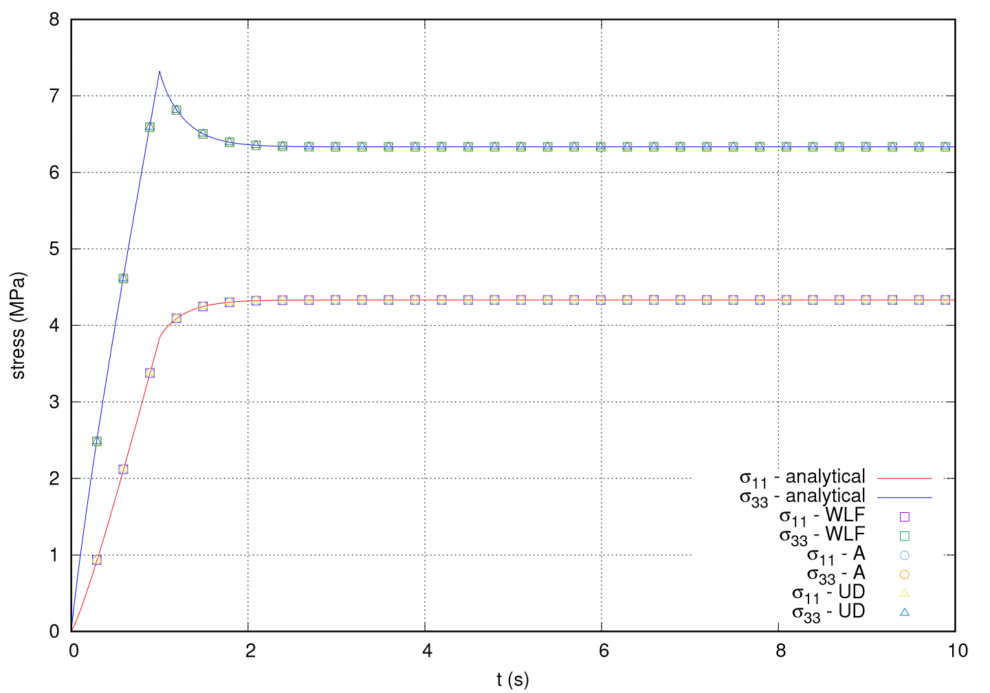
Fig. 4.149 The axial and lateral stresses with the shift factor models. (A) denotes the Arrhenius model and (UD) denotes the user defined model.

4.35.3.2. Crack Growth Kinetics

With standard viscoelasticity verified, the second test verifies the crack growth kinetics. By selecting a constant, tensile, volumetric strain rate, the frictional threshold stress intensity \(K_{0\mu}\) (4.184) reduces to \(K_{0\mu} = K_0\). Further judicious selection of the crack kinetic parameters permits an analytical solution to the crack growth rate (4.181). Note, the volumetric loading results in a linear elastic response, decoupling the viscoelasticity and crack growth kinetics. The Maxwell elements do not matter in this case. The material parameters used are shown in Table 4.60.

Table 4.60 The material properties for the viscoSCRAM model testing crack growth kinetics.

\(K\)	3460 MPa
\(G^{\infty}\)	404 MPa
\(c\)	3e-3 mm
\(a\)	1.0 mm
\(K_0\)	6920 MPa\(\sqrt{\textrm{mm}}\)
\(\mu'\)	1.16
\(m\)	2.0
\(v_{max}\)	3.0e5 mm/s
\(v_{a}\)	0.5
\(v_{b}\)	2.5
\(N\)	10
\(G^{(\kappa)}\) (MPa)	109	108	139	170	213	267	341	434	581	726
\(\tau^{(\kappa)}\) (s)	1e3	1e2	1e1	1e0	1e-1	1e-2	1e-3	1e-4	1e-5	1e-6

Three faces of a unit cube intersecting at the origin are fixed in their normal directions. A constant logarithmic strain rate is applied to the remaining three surfaces by specifying the applied displacement field as

(4.214)\[u_i = (e^{\dot{\epsilon} t} -1) X_j \delta_{ij}\]

where \(\dot{\epsilon}\) is the strain rate. Here \(\dot{\epsilon} = 0.1/\sqrt{2}\) s\(^{-1}\). The logarithmic strain rate during loading is

(4.215)\[\dot{\epsilon}_{ij} = \dot{\epsilon} \delta_{ij} .\]

The crack growth rate (4.181) becomes

(4.216)\[\begin{split}\dot{c} = \begin{cases} \left( \frac{9}{4} \frac{K}{K_0} \right)^2 \pi t^2 c & \text{for } K_I < K' \\ 100 - \frac{1}{\pi} \left( \frac{200}{9} \frac{K_0}{K}\right) \left( \frac{1}{t^2 c} \right) & \text{otherwise} . \end{cases}\end{split}\]

During stable crack growth, the analytical solution to the first-order, separable ODE (4.216)\(_1\) is

(4.217)\[c(t) = c_0 e^{\frac{1}{3} \left( \frac{9}{4} \frac{K}{K_0} \right)^2 \pi t^3} .\]

During unstable crack growth, the crack growth rate is the Chini ODE (4.216)\(_2\) which has no general closed-form solution.

An artificially high frictionless threshold stress intensity is selected, \(K_0 = 2 K\), to verify crack growth in the stable regime. The results of the analysis are shown in Fig. 4.150.

The crack size increases exponentially and the Adagio solution shows agreement with the analytical solution.

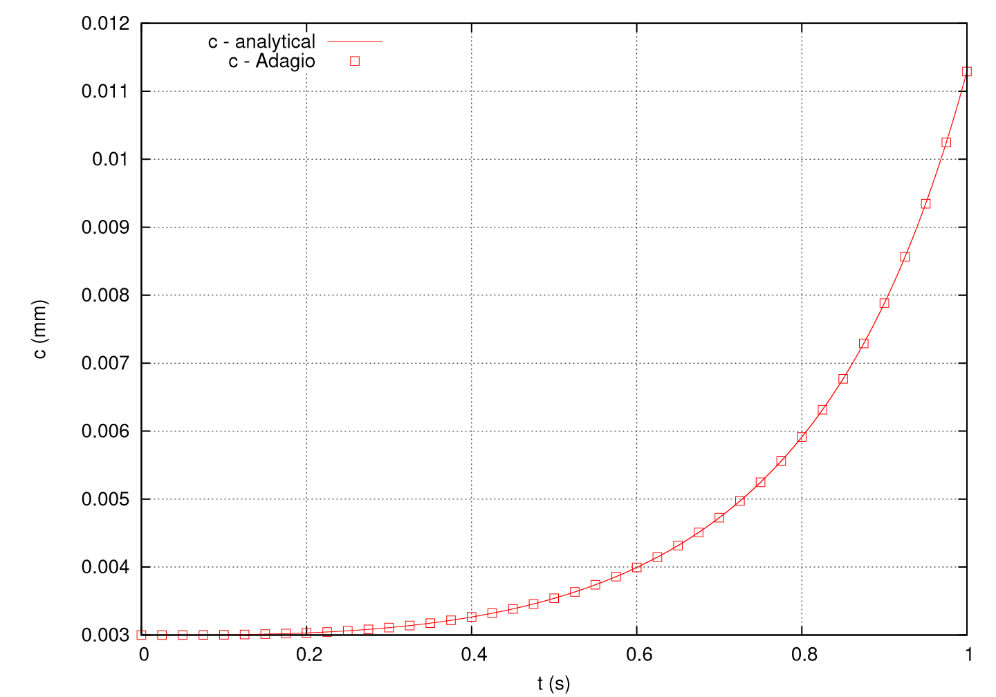
Fig. 4.150 Crack size

4.35.3.3. Uniaxial Compression

Standard viscoelasticity and crack growth during stable fracture have been verified separately. Coupled, even simple boundary-value problems do not have analytical solutions. To verify a general viscoelastic problem with crack growth, the viscoSCRAM model is compared to results from the journal article by Buechler and Luscher [[3]]. The boundary-value problem is uniaxial compression of a cylinder. The material parameters used for the code-to-code verification test are taken from the article and shown in Table 4.61.

Table 4.61 The material properties for the viscoSCRAM model tested in uniaxial compression.

\(K\)	3460 MPa
\(G^{\infty}\)	404 MPa
\(c\)	3e-3 mm
\(a\)	1.0 mm
\(K_0\)	0.03 MPa\(\sqrt{\textrm{mm}}\)
\(\mu'\)	1.16
\(m\)	10.0
\(v_{max}\)	3.0e5 mm/s
\(v_{a}\)	0.892
\(v_{b}\)	2.28
\(N\)	10
\(G^{(\kappa)}\) (MPa)	109	108	139	170	213	267	341	434	581	726
\(\tau^{(\kappa)}\) (s)	1e3	1e2	1e1	1e0	1e-1	1e-2	1e-3	1e-4	1e-5	1e-6

The results of the analysis are shown in Fig. 4.151. The axial stress increases linearly and then begins to soften due to the accumulation of damage as crack growth occurs. The simulation is for the curve corresponding to the time step \(\Delta t = 0.0625\) s in the journal article. The Adagio implementation shows agreement with the journal implementation.

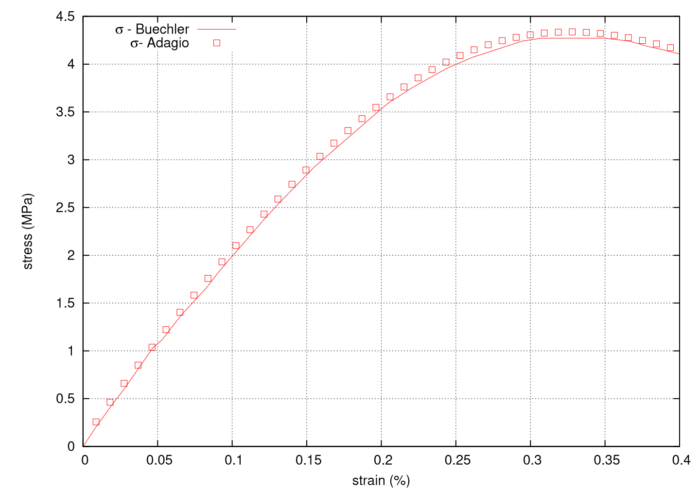
Fig. 4.151 Uniaxial compression

4.35.3.4. Viscoplasticity

Uniaxial tension

For the viscoplastic component of the viscoplastic-viscoSCRAM model, the first verification boundary-value problem is uniaxial tension of a unit cube. Zeroing the initial crack size, \(c = 0\), and setting the number of Maxwell elements to zero, reduces the model to the purely viscoplastic model. The crack growth kinetic parameters do not matter in this case. The material parameters used are shown in Table 4.62.

Three faces of a unit cube intersecting at the origin are fixed in their normal directions. A constant logarithmic strain rate ramp load followed by a holding period is applied to the cube in the \(x_1\)-direction by specifying the applied displacement in this direction as

(4.218)\[\begin{split}u_1 = \begin{cases} (e^{\beta \left( \frac{\sigma_y}{E} \right) \left( \frac{t}{t_L}\right) } -1) X_1 & \text{for } t < t_L \\ (e^{\beta \left( \frac{\sigma_y}{E} \right)} -1) X_1 & \text{otherwise} \end{cases}\end{split}\]

where \(\beta\) is a scaling parameter and \(t_L\) is the ramp loading time. Here \(\beta = \frac{E}{\sigma_y}\) and \(t_L = 1\) s which corresponds to a \(100\%\) logarithmic axial strain. The logarithmic strain in the applied displacement direction is

(4.219)\[\begin{split}\epsilon_{11} = \begin{cases} \beta \left( \frac{\sigma_y}{E} \right) \left( \frac{t}{t_L}\right) & \text{for } t < t_L \\ \beta \left( \frac{\sigma_y}{E} \right) & \text{otherwise} . \end{cases}\end{split}\]

Table 4.62 The material properties for the viscoplastic model tested in uniaxial tension.

\(K\)	5.0 MPa
\(G^{\infty}\)	1.0 MPa
\(c\)	0.0 mm
\(N\)	0
\(A\)	1.0
\(\sigma_y\)	2.0 MPa
\(B\)	1.0
\(\tilde{\tau}\)	0.8 s
\(\sigma_0\)	1.0 MPa
\(\tilde{m}\)	1.0

In the Drucker-Prager flow rule, set \(\tilde{m} = 1\) so that the plastic flow rate is linear in stress and given by

(4.220)\[\dot{\lambda} = \frac{1}{\tilde{\tau}} \left( \frac{f}{\sigma_0} \right) .\]

For uniaxial tension, the analytical Cauchy stress in the loading direction is

(4.221)\[\begin{split}\sigma_{11}(t) = \begin{cases} \frac{\beta \sigma_y}{t_L} t & \text{for } t \le t_y \\ \left( \frac{c_2}{c_1} \right) + \left( \frac{c_3}{c_1} \right) + \left[ \frac{3 \sigma_y}{(3+A)t_L} - \left( \frac{c_2}{c_1} \right) - \left( \frac{c_3}{c_1} \right) \right] e^{-c_1(t-t_y)} & \text{for } t_y < t < t_L \\ \left( \frac{c_2}{c_1} \right) + \left( \frac{c_3}{c_1} \right) e^{-c_1(t-t_L)} + \left[ \frac{3 \sigma_y}{(3+A)t_L} - \left( \frac{c_2}{c_1} \right) - \left( \frac{c_3}{c_1} \right) \right] e^{-c_1(t-t_y)} & \text{for } t \ge t_L , \\ \end{cases}\end{split}\]

where

(4.222)\[\begin{split}c_1 &= E \left( \frac{1}{\tilde{\tau} \sigma_0} \right) \left[ (1 + \frac{1}{9} A \cdot B) + \frac{1}{3} (A+B) \right] \\ c_2 &= E \left( \frac{1}{\tilde{\tau} \sigma_0} \right) (\sigma_y) (1 + \frac{1}{3}B) \\ c_3 &= \frac{\beta \sigma_y}{t_L} ,\end{split}\]

and

(4.223)\[t_y = \frac{3 t_L}{\beta (3+A)}.\]

Here, \(t_y\) is the time at yielding.

The results of the analysis, using the implicit solution scheme with a timestep of \(\Delta t = 0.025\) s, are shown in Fig. 4.152. The Adagio solition shows agreement with the analytical solution.

The time at yielding is \(t_y = 0.5333\) s. The axial stress is linear elastic until this time and then the response is viscoplastic until the end of the loading period, \(t_L = 1.0\) s. After the loading period, axial strain is held fixed; stress relaxes asymptotically to

(4.224)\[\sigma_{11}^{\infty} = \sigma_{11}(t \rightarrow \infty) = \frac{c_2}{c_1} = \left( \frac{9+3B}{9+A \cdot B + 3(A+B) } \right) \sigma_y ,\]

or, for the selected material parameters, \(\sigma_{11}^{\infty} = 0.75 \sigma_y\).

As the relaxation time \(\tilde{\tau}\) decreases, the stress relaxes more quickly to \(\sigma_{11}^{\infty}\). In the limit, as \(\tilde{\tau} \rightarrow 0\), the viscoplastic stress is relaxed immediately and the solution converges to the rate independent plastic solution. Also, as the pressure dependence of the yield surface is reduced, \(A \rightarrow 0\), the yield surface reduces to the von Mises yield surface where \(\sigma_{11}^{\infty} = \sigma_y\). If the pressure dependence of the flow surface is also eliminated; that is, \(A = B = 0\), then the flow direction is associative von Mises and as \(\tilde{\tau} \rightarrow 0\), the solution converges to rate independent J2 plasticity.

Fig. 4.152 Uniaxial tension

Simple shear

For the viscoplastic component of the viscoplastic-viscoSCRAM model, the second verification boundary-value problem is simple shear of a unit cube. Again, zeroing the initial crack size, \(c = 0\), and setting the number of Maxwell elements to zero, reduces the model to the purely viscoplastic model. The crack growth kinetic parameters do not matter in this case. The material parameters used are shown in Table 4.63.

The \(x_2=0\) face of a unit cube is fixed. The faces with \(x_3\)-normals are fixed in the normal directions. A constant strain rate ramp load followed by a holding period is applied to the cube in the \((x_1x_2)\)-plane by specifying the applied displacement in the \(x_1\)-direction as

(4.225)\[\begin{split}u_1 = \begin{cases} \beta \left( \frac{t}{t_L}\right) X_2 & \text{for } t < t_L \\ \beta X_2 & \text{otherwise} . \end{cases}\end{split}\]

where \(\beta\) is a scaling parameter and \(t_L\) is the ramp loading time. Here \(\beta = 0.05\) and \(t_L = 1\) s which corresponds to a \(2.5\%\) shear strain. These parameters were selected to satisfy the small deformation assumption necessary for the analytical solution. The shear strain is

(4.226)\[\begin{split}\epsilon_{12} = \begin{cases} \frac{1}{2} \beta \left( \frac{t}{t_L}\right) & \text{for } t < t_L \\ \frac{1}{2} \beta & \text{otherwise} . \end{cases}\end{split}\]

Table 4.63 The material properties for the viscoplastic model tested in simple shear.

\(K\)	5.0 MPa
\(G^{\infty}\)	1.0 MPa
\(c\)	0.0 mm
\(N\)	0
\(A\)	1.0
\(\sigma_y\)	\(\sqrt{3}/40\) MPa
\(B\)	0.0
\(\tilde{\tau}\)	0.8 s
\(\sigma_0\)	1.0 MPa
\(\tilde{m}\)	1.0

For simple shear, the analytical Cauchy stress in the shear plane is

(4.227)\[\begin{split}\sigma_{12}(t) = \begin{cases} \frac{\beta G}{t_L} t & \text{for } t \le t_y \\ \left( \frac{c_2}{c_1} \right) + \left( \frac{c_3}{c_1} \right) + \left[ \frac{\sigma_y}{\sqrt{3}} - \left( \frac{c_2}{c_1} \right) - \left( \frac{c_3}{c_1} \right) \right] e^{-c_1(t-t_y)} & \text{for } t_y < t < t_L \\ \left( \frac{c_2}{c_1} \right) + \left( \frac{c_3}{c_1} \right) e^{-c_1(t-t_L)} + \left[ \frac{\sigma_y}{\sqrt{3}} - \left( \frac{c_2}{c_1} \right) - \left( \frac{c_3}{c_1} \right) \right] e^{-c_1(t-t_y)} & \text{for } t \ge t_L , \\ \end{cases}\end{split}\]

where

(4.228)\[c_1 = 3 G \left( \frac{1}{\tilde{\tau} \sigma_0} \right), \qquad c_2 = \sqrt{3} G \left( \frac{1}{\tilde{\tau} \sigma_0} \right) (\sigma_y), \qquad c_3 = \frac{\beta G}{t_L} ,\]

and

(4.229)\[t_y = \frac{\sigma_y t_L}{\sqrt{3} \beta G}.\]

Here, \(t_y\) is the time at yielding.

The results of the analysis, using the implicit solution scheme, are shown in Fig. 4.153. The Adagio solition shows agreement with the analytical solution.

The time at yielding is \(t_y = 0.5\) s. The shear stress is linear elastic until this time and then the response is viscoplastic until the end of the loading period, \(t_L = 1.0\) s. After the loading period, shear strain is held fixed; stress relaxes asymptotically to

(4.230)\[\sigma_{12}^{\infty} = \sigma_{12}(t \rightarrow \infty) = \frac{c_2}{c_1} = \frac{\sigma_y}{\sqrt{3} }.\]

As the relaxation time \(\tilde{\tau}\) decreases, the stress relaxes more quickly to \(\sigma_{12}^{\infty}\). In the limit, as \(\tilde{\tau} \rightarrow 0\), the viscoplastic stress is relaxed immediately and the solution converges to the rate independent plastic solution. For the small deformation simple shear problem, with the flow direction pressure independent (\(B=0\)), no normal stresses are developed. The yield surface is then independent of the pressure coefficient \(A\) and as \(\tilde{\tau} \rightarrow 0\), the solution converges to rate independent J2 plasticity.

Fig. 4.153 Simple shear

4.35.4. User Guide

BEGIN PARAMETERS FOR MODEL VISCOPLASTIC_VISCOSCRAM
  #
  # Elastic constants
  #
  BULK MODULUS   = <real>
  SHEAR MODULUS  = <real>
  #
  # Crack growth kinetics
  #
  CRACK SIZE        = <real>
  CRACK NORM        = <real>
  STRESS INTENSITY  = <real>
  FRICTION          = <real>
  CRACK SHAPE       = <real>
  CRACK SPEED MAX   = <real>
  CRACK SPEED A     = <real>
  CRACK SPEED B     = <real>
  CRACK SPEED C     = <real> (1.0)
  #
  # Viscoelasticity
  #
  NME    = <integer>
  SHEAR  = <real_list>
  TAU    = <real_list>
  #
  # Time-temperature superposition
  #
  SHIFT FACTOR MODEL = <string> NONE | WLF | ARRHENIUS | USER_DEFINED (NONE)

  SHIFT FACTOR MODEL = WLF
    WLF C1 = <real>
    WLF C2 = <real>
    REFERENCE TEMPERATURE = <real>

  SHIFT FACTOR MODEL = ARRHENIUS
    NORM ACTIVATION ENERGY = <real>
    REFERENCE TEMPERATURE  = <real>

  SHIFT FACTOR MODEL = USER_DEFINED
    SHIFT FACTOR FUNCTION = <string>
  #
  # Viscoplasticity
  #
  VISCOPLASTIC MODEL = <string> NONE | EXPLICIT | IMPLICIT (NONE)

  VISCOPLASTIC MODEL = EXPLICIT | IMPLICIT
  F A           = <real>
  F YIELD       = <real>
  G B           = <real>
  FLOW TAU      = <real>
  FLOW SIGMA    = <real>
  FLOW M        = <real>

  TOLERANCE NR  = <real> (1.0e-8)

END [PARAMETERS FOR VISCOPLASTIC_VISCOSCRAM]

Output variables available for this model are listed in Table 4.64.

The equivalent plastic strain \(\bar{\epsilon}^p\), plastic work \(Q\), and plastic work rate \(\dot{Q}\) output variables are defined as:

\[\bar{\epsilon}^p = \int_0^t \sqrt{\frac{2}{3} \dot{\varepsilon}_{ij}^p \dot{\varepsilon}_{ij}^p } \,dt , \qquad Q = \int_0^t \sigma_{ij} \dot{\varepsilon}_{ij}^p \,dt , \qquad \dot{Q} = \sigma_{ij} \dot{\varepsilon}_{ij}^p .\]

Table 4.64 State Variables for VISCOSCRAM EXPLICIT Model

Name	Description
C	crack size
CDOT	crack velocity
CSTABILITY	crack stability ratio, \(K_I/K'\)
DAMAGE	damage, \(D\)
ASHIFT	shift factor, \(a_T(T)\)
EQPS	equivalent plastic strain, \(\bar{\varepsilon}^p\)
PLASTIC_WORK	plastic work, \(Q\)
PLASTIC_WORK_RATE	plastic work rate, \(\dot{Q}\)

---

[1]

J.K. Dienes. A statistical-theory of fragmentation processes. Mechanics of Materials, 4(3-4):325–335, 1985.

[2]

R.M. Hackett and J.G. Bennett. An implicit finite element material model for energetic particulate composite materials. Int. J. Numer. Meth. Engng., 49:1191–1209, 2000.

[3] (1,2)

M.A. Buechler and D.J. Luscher. A semi-implicit integration scheme for a combined viscoelastic-damage model of plastic bonded explosives. Int. J. Numer. Meth. Engng., 99:54–78, 2014.

[4]

C. Vignes and K. Long. Viscoplastic-viscoSCRAM model for particulate composite materials. Technical report, SAND2021- In review., Sandia National Laboratories, Albuquerque, New Mexico 87185 and Livermore, California 94550, September 2021.

[5]

M.A. Buechler. Viscoelastic-viscoplastic combined hardening constitutive model based on the Drucker Prager yield and flow potentials. Technical report, LA-UR-12-24895, Los Alamos National Laboratory, Los Alamos, New Mexico 87545, 2012.

[6]

M.A. Buechler. Viscoelastic viscoplastic damage model development, parameter estimation, and comparison to PBX9501 experimental data. Technical report, LA-UR-13-27547, Los Alamos National Laboratory, Los Alamos, New Mexico 87545, 2013.

[7]

M. Kojić and K.J. Bathe. Inelastic Analysis of Solids and Structures. Springer, 2005.

[8]

S. Marques and G.J. Creus. Computational Viscoelasticity. Springer, 2012.

[9]

T.J.R Hughes and R.L. Taylor. Unconditionally stable algorithms for quasi-static elasto/visco-plastic finite element analysis. Comput Struct, 8:169–173, 1978.