4.7. Elastic-Plastic Model

4.7.1. Theory

The elastic-plastic model is a hypoelastic, rate-independent linear hardening plasticity model. The rate form of the constitutive equation assumes an additive split of the rate of deformation into an elastic and plastic part

(4.19)\[D_{ij} = D^{\text{e}}_{ij} + D^{\text{p}}_{ij}\]

The stress rate only depends on the elastic strain rate in the problem

(4.20)\[\stackrel{\circ}{\sigma}_{ij} = \mathbb{C}_{ijkl}D^{\text{e}}_{kl}\]

where \(\mathbb{C}_{ijkl}\) are the components of the fourth-order, isotropic elasticity tensor.

The key to the model is finding the plastic rate of deformation. For associated flow the plastic rate of deformation is in a direction normal to the yield surface. The yield surface is given by

(4.21)\[f\left(\sigma_{ij},\alpha_{ij},\bar{\varepsilon}^{p}\right) = \phi\left(\sigma_{ij},\alpha_{ij}\right) - \bar{\sigma}\left(\bar{\varepsilon}^{p}\right) = 0\]

where \(\phi\) is the effective stress, \(\alpha_{ij}\) are the components of the back stress (used with kinematic hardening), and \(\bar{\sigma}\) is the hardening function which is a function of an internal state variable, the equivalent plastic strain \(\bar{\varepsilon}^{p}\). An example of such a yield surface (plotted in the deviatoric \(\pi\)-plane) is presented below in Fig. 4.16. The isotropy of the yield surface is clearly evident.

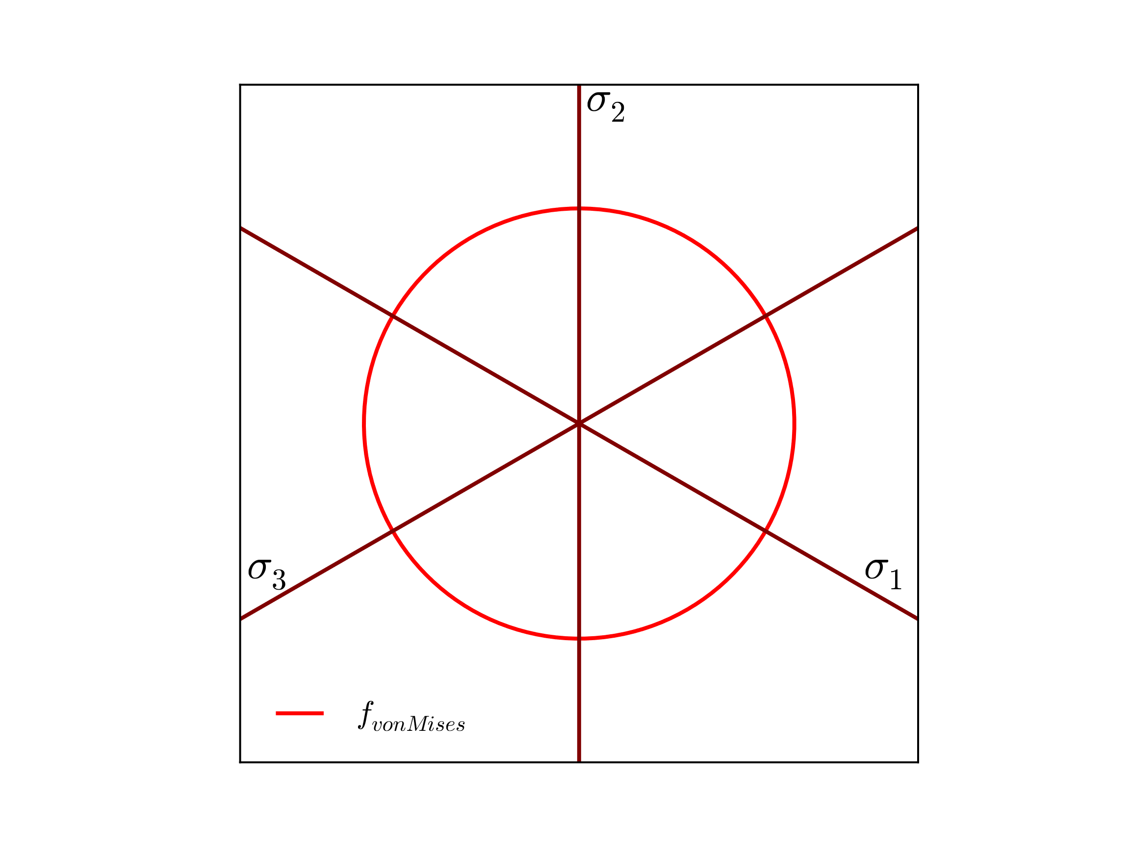
Fig. 4.16 Example von Mises yield surface (\(J_2\)) used by the elastic-plastic model presented in the deviatoric \(\pi\)-plane. In this case the surface is plotted for \(\alpha_{ij}=0\) and \(\bar{\varepsilon}^p=0\).

For the elastic plastic model a linear hardening law is assumed

(4.22)\[\bar{\sigma} = \sigma_{y} + H^{\prime}\bar{\varepsilon}^{p}\]

where \(\sigma_{y}\) is the yield stress and \(H^{\prime}\) is the hardening modulus.

If the stress state is such that \(f < 0\), the the behavior of the material is elastic; if the stress state is such that \(f = 0\) and \(\dot{f} < 0\), i.e. the strain rate brings the stress inside the yield surface, then the behavior of the material is elastic; if the stress state is such that \(f = 0\) and \(\dot{f} > 0\), i.e. the strain rate brings the stress outside the yield surface, then plastic deformation occurs.

We assume associated flow in this model, which gives the plastic rate of deformation

(4.23)\[D^{\text{p}}_{ij} = \dot{\gamma}\frac{\partial\phi}{\partial\sigma_{ij}}\]

where \(\dot{\gamma}\) is the consistency parameter. For the elastic-plastic model the yield surface is assumed to be a von Mises yield surface with a back stress tensor to denote the center of the yield surface. The effective stress for a von Mises yield surface is

(4.24)\[\phi\left(\sigma_{ij}\right) = \sqrt{\frac{3}{2}\xi_{ij}\xi_{ij}} \;\;\; ; \;\;\; \xi_{ij} = s_{ij} - \alpha_{ij}\]

where \(s_{ij}\) are the components of the deviatoric stress tensor

(4.25)\[s_{ij} = \sigma_{ij} - \frac{1}{3}\delta_{ij}\sigma_{kk}\]

and \(\alpha_{ij}\) are the components of the back stress tensor, another internal state variable.

The equivalent plastic strain is found through equating the rate of plastic work

(4.26)\[\begin{split}\dot{W}^{p} = \sigma_{ij}D^{\text{p}}_{ij} = \bar{\sigma}\dot{\bar\varepsilon}^{p} \;\;\; \rightarrow \;\;\; \dot{\bar\varepsilon}^{p} = \dot{\gamma} \nonumber \\ \bar{\varepsilon}^{p} = \int_{0}^{t} \dot{\gamma} dt \nonumber\end{split}\]

Finally, the model allows for kinematic hardening through the back stress. The back stress is a symmetric, deviatoric rank two tensor that evolves in the following manner

(4.27)\[\dot{\alpha}_{ij} = \frac{2}{3}\left( 1-\beta \right) H^{\prime} D_{ij}^{\text{p}}\]

The radius of the yield surface can be defined, \(R = \sqrt{\xi_{ij}\xi_{ij}}\). The evolution of the radius of the yield surface is given by

(4.28)\[\dot{R} = \sqrt{\frac{2}{3}} \beta H^{\prime} \dot{\bar\varepsilon}^{p}\]

In (4.27) and (4.28) the parameter \(\beta \in [0,1]\) distributes the hardening between isotropic and kinematic hardening. If \(\beta = 1\) the hardening is isotropic, if \(\beta = 0\) the hardening is kinematic, and if \(\beta\) is between 0 and 1 the hardening is a combination of isotropic and kinematic.

4.7.2. Implementation

The elastic-plastic linear hardening model is implemented using a predictor-corrector algorithm. First, an elastic trial stress state is calculated. This is done by assuming that the rate of deformation is completely elastic

\[T^{tr}_{ij} = T^{n}_{ij} + \Delta t \left( \lambda\delta_{ij} d_{kk} + 2\mu d_{ij} \right)\]

The trial stress state can be decomposed into a pressure and a deviatoric stress

\[p^{tr} = \frac{1}{3} T^{tr}_{kk} \;\;\; ; \;\;\; s^{tr}_{ij} = T^{tr}_{ij} - p^{tr}\delta_{ij}\]

The difference between the deviatoric trial stress state and the back stress is compared to the current radius of the yield surface

\[\xi^{tr}_{ij} = s^{tr}_{ij} - \alpha^{n}_{ij} \;\;\; ; \;\;\; \xi_{tr}^{2} = \xi^{tr}_{ij}\xi^{tr}_{ij}\]

If \(\xi_{tr}^{2} < R^2\) then the strain rate is elastic and the stress update is finished. If \(\xi_{tr}^{2} > R^2\) then plastic deformation has occurred. The algorithm then needs to determine the extent of plastic deformation.

The normal to the yield surface, \(N_{ij}\) is assumed to lie in the direction of the trial stress state. This gives us the following expression for \(N_{ij}\)

\[N_{ij} = \frac{\xi_{ij}^{tr}}{\|\xi_{ij}^{tr}\|}\]

In what follows the change in the yield surface is assumed to be a linear combination of isotropic and kinematic hardening, i.e. the yield surface grows and or moves. Using a backward Euler algorithm the final deviatoric stress state is

\[s^{n+1}_{ij} = s^{tr}_{ij} - \Delta t \, 2\mu d^{\text{p}}_{ij}\]

where the plastic strain increment is

\[\Delta t \, d^{p}_{ij} = \sqrt{\frac{3}{2}} \Delta\bar{\varepsilon}^{p}N_{ij}\]

The updated back stress is

\[\alpha^{n+1}_{ij} = \alpha^{n}_{ij} + \sqrt{\frac{2}{3}} \left( 1-\beta \right) \left( H^{\prime}\Delta\bar{\varepsilon}^{p} \right) N_{ij}\]

and the updated radius of the yield surface is

\[R^{n+1} = R^{n} + \beta \sqrt{\frac{2}{3}} \left( H^{\prime}\Delta\bar{\varepsilon}^{p} \right)\]

Combining these expressions we get an equation for the change in the equivalent plastic strain over the load step

\[\left( 3\mu + H^{\prime} \right) \Delta\bar{\varepsilon}^{p} = \sqrt{\frac{3}{2}} \left( \| \xi_{ij}^{tr} \| - R^{n} \right) \;\;\; ; \;\;\; \xi^{tr}_{ij} = s^{tr}_{ij} - \alpha^{n}_{ij}\]

With \(\Delta\bar{\varepsilon}^{p}\) we can update the stress and the internal state variables.

4.7.3. Verification

The elastic-plastic material model is verified for a number of loading conditions. The elastic properties used in these analyses are \(E = 70\) GPa and \(\nu = 0.25\). The hardening parameters are \(\sigma_{y} = 200\) MPa, \(H' = 500\) MPa, and \(\beta = 1\). By setting \(\beta = 1\) the hardening is isotropic.

4.7.3.1. Uniaxial Stress

The elastic-plastic model is tested in uniaxial tension. The test looks at the stress, strain, and equivalent plastic strain and compares these values against analytical results for the same problem. The model is tested in uniaxial stress in the \(x\) (\(x_{1}\)), directions.

For the uniaxial stress problem, the only non-zero stress component is \(\sigma_{11}\). In the analysis that follows \(\sigma_{11} = \sigma\). There are three non-zero strain components, \(\varepsilon_{11}\), \(\varepsilon_{22}\), and \(\varepsilon_{33}\). In the analysis that follows \(\varepsilon_{11} = \varepsilon\). Furthermore, the axial elastic stress, \(\varepsilon_{11}^{\text{e}} = \sigma/E\) will be denoted by \(\varepsilon^{\text{e}}\).

4.7.3.1.1. Axial Stresses

The uniaxial stress calculated by the model in Adagio is compared to an analytical solution. For uniaxial loading in the \(x_{1}\) direction, the effective stress is

\[\phi = \sigma\]

If the stress state is on the yield surface, then \(\phi = \bar{\sigma}\left(\bar{\varepsilon}^{p}\right)\), so the axial stress, as a function of the hardening function, is

(4.29)\[\sigma = \bar{\sigma}\left(\bar{\varepsilon}^{p}\right) = \sigma_{y} + H^{\prime} \bar{\varepsilon}^{p}\]

The stress state can be calculated from the hardening law and the anisotropy parameters.

To evaluate the axial stress we need the equivalent plastic strain as a function of the axial strain. If we equate the rate of plastic work we get

\[\bar{\sigma} \dot{\bar{\varepsilon}}^{p} = \sigma \left( \dot\varepsilon - \dot\varepsilon^{\text{e}} \right) \;\;\; \rightarrow \;\;\; \dot{\bar{\varepsilon}}^{p} = \dot\varepsilon - \dot\varepsilon^{\text{e}}\]

which, when integrated, gives us an equation for the equivalent plastic strain

(4.30)\[\bar{\varepsilon}^{p} = \frac{E\varepsilon - \sigma_{y}}{E + H^{\prime}}\]

The equivalent plastic strain can then be used in (4.50) to find the axial stress, \(\sigma\)

(4.31)\[\sigma = \frac{\sigma_{y} + H^{\prime}\varepsilon}{1 + H^{\prime}/E}\]

The axial stresses is shown in Fig. 4.17.

4.7.3.1.2. Lateral Strains

For the lateral strains we need the plastic strains and therefore the normal to the yield surface. The components of the normal to the yield surface are

\[\frac{\partial\phi}{\partial \sigma_{11}} = 1 \;\;\; ; \;\;\; \frac{\partial\phi}{\partial \sigma_{22}} = \frac{\partial\phi}{\partial \sigma_{33}} = -\frac{1}{2}\]

The elastic axial and lateral strain components are

\[\varepsilon^{\text{e}}_{11} = \frac{\sigma}{E} = \varepsilon^{\text{e}} \;\;\; ; \;\;\; \varepsilon^{\text{e}}_{22} = \varepsilon^{\text{e}}_{33} = -\nu\frac{\sigma}{E} = -\nu\varepsilon^{\text{e}}\]

The plastic axial strain component is

\[\varepsilon^{\text{p}}_{11} = \varepsilon_{11} - \frac{\sigma}{E} = \varepsilon - \varepsilon^{\text{e}}\]

which comes from the additive decomposition of the strain rates. Using the equivalent plastic strain (4.51) we can find the lateral plastic strain components

\[\varepsilon^{\text{p}}_{22} = \varepsilon^{\text{p}}_{33} = - \frac{1}{2}\left( \varepsilon - \varepsilon^{\text{e}} \right)\]

The lateral {em total} stain components prior to yield are \(\varepsilon_{22} = \varepsilon_{33} = -\nu \varepsilon\). After yield they are

\[\varepsilon_{22} = \varepsilon_{33} = -\nu \varepsilon^{\text{e}} - \frac{1}{2} \bar{\varepsilon}^{p}\]

where \(\varepsilon^{\text{e}} = \sigma/E\).

Results are shown in Fig. 4.18.

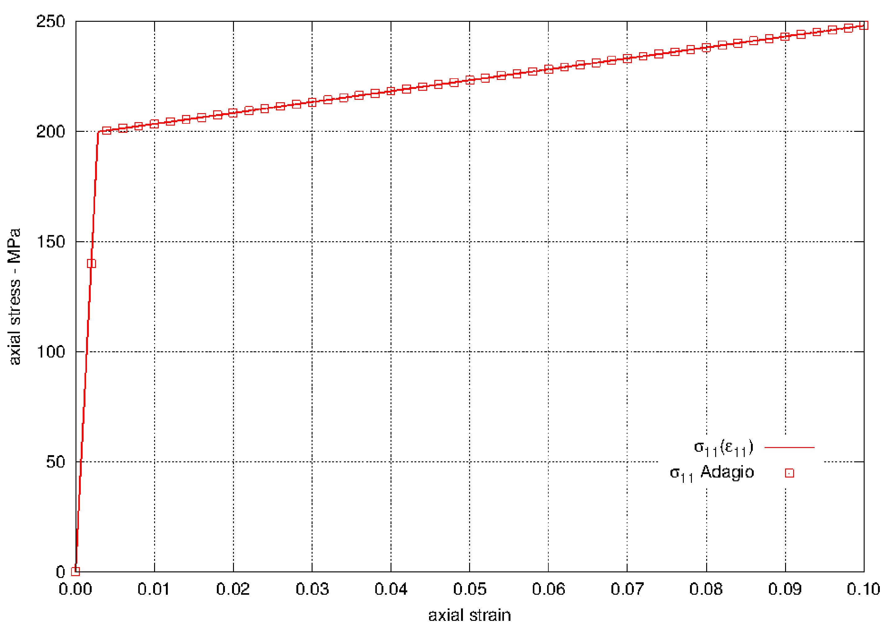
Fig. 4.17 Axial stress for loading in the \(x_{1}\) direction for the elastic-plastic model with linear hardening.

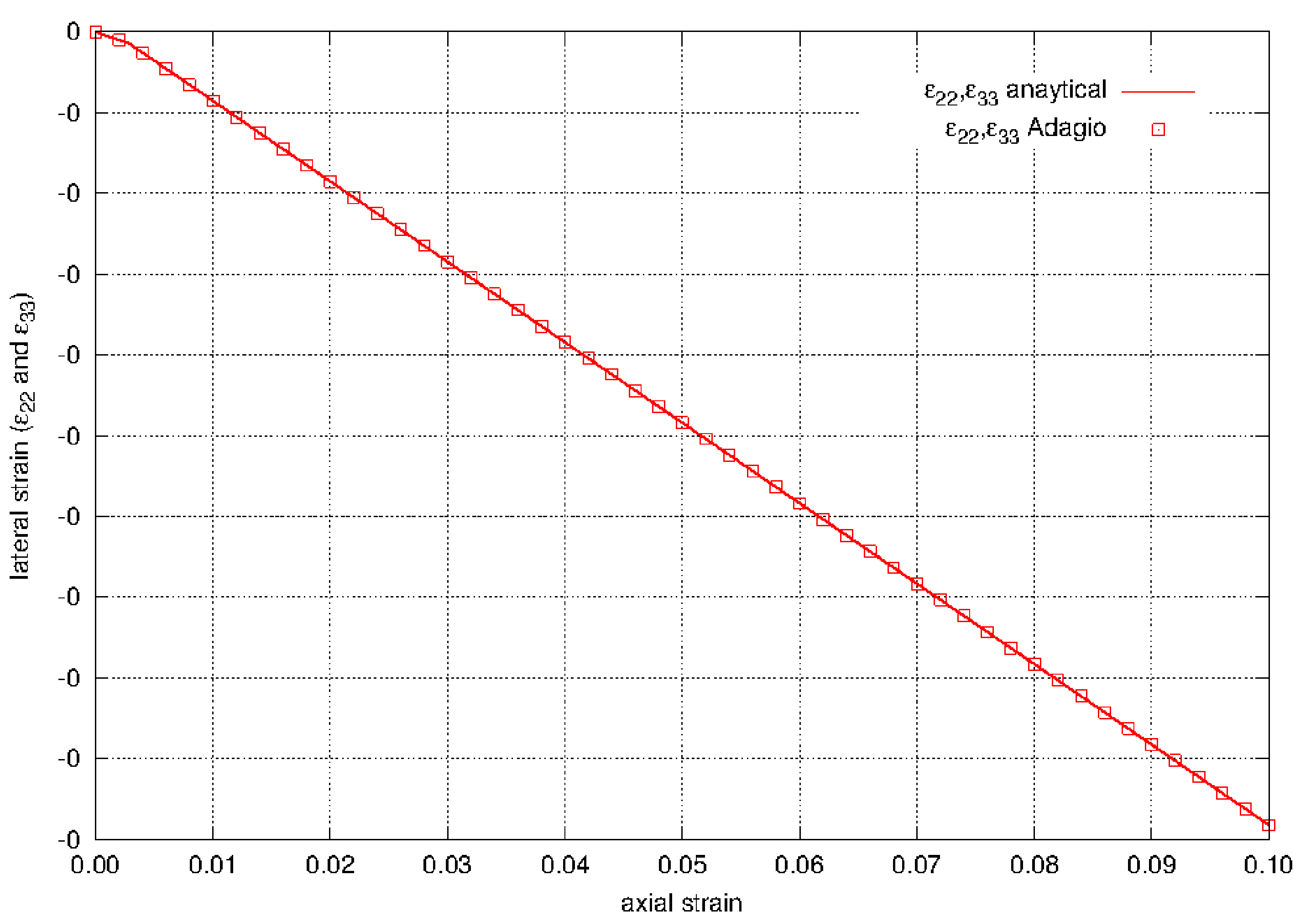
Fig. 4.18 Lateral strains for uniaxial stress loading in the \(x_{1}\) direction for the elastic-plastic model with linear hardening.

4.7.3.2. Pure Shear

The shear stress calculated by the elastic-plastic model in Adagio is compared to analytical solutions. Considering pure shear with respect to the \(x_{1}\)-\(x_{2}\) axes, the only non-zero shear stress is \(\sigma_{12}\), and the only non-zero shear strain will be \(\varepsilon_{12}\) For pure shear with respect to the \(x_{1}\)-\(x_{2}\) axes, the effective stress is

\[\phi = \sqrt{3} \, \sigma_{12}\]

If the stress state is on the yield surface, then \(\phi = \bar{\sigma}\left(\bar{\varepsilon}^{p}\right)\), so the shear stress is

(4.32)\[\sigma_{12} = \frac{\bar{\sigma}\left(\bar{\varepsilon}^{p}\right)}{\sqrt{3}}\]

Using this, the pure shear stress state can be calculated from the hardening law and the anisotropy parameters.

To evaluate the shear stress we need the equivalent plastic strain as a function of the shear strain. If we equate the rate of plastic work we get

\[\bar{\sigma}\dot{\bar{\varepsilon}}^{p} = 2 \sigma_{12} \left( \dot{\varepsilon}_{12} - \dot{\varepsilon}_{12}^{e} \right) \;\;\; \rightarrow \;\;\; \dot{\bar{\varepsilon}}^{p} = \frac{2}{\sqrt{3}} \left( \dot{\varepsilon}_{12} - \dot{\varepsilon}_{12}^{e} \right)\]

which, when integrated, gives us an implicit equation for the equivalent plastic strain

\[\bar{\varepsilon}^{p} = \frac{2}{\sqrt{3}} \left( \varepsilon_{12} - \frac{\bar{\sigma}\left(\bar{\varepsilon}^{p}\right)}{\sqrt{3}\,G} \right)\]

The equivalent plastic strain can now be used to find the shear stress.

4.7.3.2.1. Boundary Conditions for Pure Shear

The deformation gradient that gives pure shear for loading relative to the \(x_{1}\)-\(x_{2}\) axes is

\[\begin{split}\left[ {\bf F} \right] = \begin{bmatrix} \frac{1}{2} \left( \lambda + \lambda^{-1} \right) & \frac{1}{2} \left( \lambda - \lambda^{-1} \right) & 0 \\ \\ \frac{1}{2} \left( \lambda - \lambda^{-1} \right) & \frac{1}{2} \left( \lambda + \lambda^{-1} \right) & 0 \\ \\ 0 & 0 & 1 \end{bmatrix} \;\;\; \rightarrow \;\;\; \left[ {\boldsymbol{\varepsilon}} \right] = \begin{bmatrix} 0 & \varepsilon & 0 \\ \\ \varepsilon & 0 & 0 \\ \\ 0 & 0 & 0 \end{bmatrix} \;\;\; ; \;\;\; \varepsilon = \ln\lambda\end{split}\]

For loading relative to the \(x_{2}\)-\(x_{3}\) axes and the \(x_{3}\)-\(x_{1}\) axes the boundary conditions are modified appropriately.

4.7.3.2.2. Results

The results for the elastic-plastic model loaded in pure shear are shown in Fig. 4.19. We see that the stress strain curves in pure shear as calculated by Adagio follow the expected stress strain curves. All other stress and strain components for the three problems are zero.

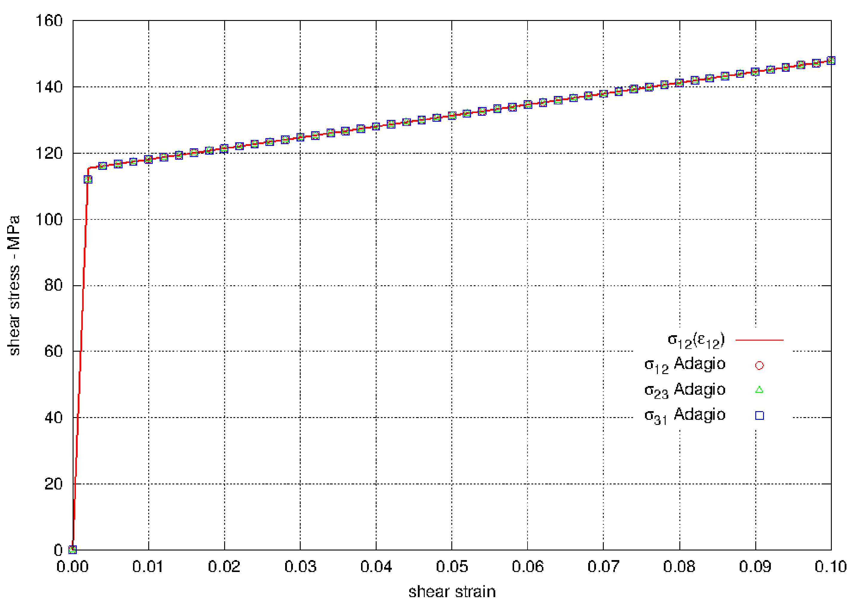
Fig. 4.19 Results are for shear in the \(x_{1}\)-\(x_{2}\) plane, \(x_{2}\)-\(x_{3}\) plane, and \(x_{3}\)-\(x_{1}\) plane.

4.7.4. User Guide

BEGIN PARAMETERS FOR MODEL ELASTIC_PLASTIC
  #
  # Elastic constants
  #
  YOUNGS MODULUS = <real>
  POISSONS RATIO = <real>
  SHEAR MODULUS  = <real>
  BULK MODULUS   = <real>
  LAMBDA         = <real>
  TWO MU         = <real>
  #
  # Hardening Behavior
  #
  YIELD STRESS      = <real>
  BETA              = <real>
  HARDENING MODULUS = <real>
END [PARAMETERS FOR MODEL ELASTIC_PLASTIC]

In the above command blocks:

• The elastic constants describe both the pre-yield behavior of the model and the slope of post yield unloading.

• The yield stress, the stress at which yield first initiates, is defined with the YIELD STRESS command line.

• The hardening modulus, the slope of the post yield hardening curve, is defined with the HARDENING MODULUS command line.

• The beta parameter defines if hardening is isotropic or kinematic.

Output variables available for this model are listed in Table 4.5 and Table 4.6. For information about the elastic-plastic model, consult [[1]].

Table 4.5 State Variables for ELASTIC PLASTIC Model

Name	Description
EQPS	equivalent plastic strain, \(\bar{\varepsilon}^{p}\)
RADIUS	radius of the yield surface, \(R\)
BACK_STRESS	back stress (symmetric tensor), \(\alpha_{ij}\)

Table 4.6 State Variables for ELASTIC PLASTIC Model for Shells

Name	Description
EQPS	equivalent plastic strain, \(\bar{\varepsilon}^{p}\)
TENSILE_EQPS	equivalent plastic strain only accumulated when the material is in tension (trace of stress tensor is positive)
RADIUS	radius of the yield surface, \(R\)
BACK_STRESS	back stress (symmetric tensor), \(\alpha_{ij}\)
ITERATIONS	radial return iterations
ERROR	error in plane stress iterations
PS_ITER	plane stress iterations
TSTRAIN	integrated thickness strain

---

[1]

C.M. Stone. SANTOS – a two-dimensional finite element program for the quasistatic, large deformation, inelastic response of solids. Technical Report SAND90-0543, Sandia National Laboratories, Albuquerque, NM, 1996. \href http://infoserve.sandia.gov/sand_doc/1990/900543.pdfpdf.