4.18. Modular Plane Stress Plasticity Model

4.18.1. Theory

Like the plane stress plasticity model of Section 4.17, the modular plane stress plasticity (MPSP) model is a plane stress implementation of a \(J_2\) plasticity formulation largely following and motivated by the works of Simo and Taylor [[1]] and Simo and Hughes [[2]]. However, the modular plane stress plasticity model differs from those prior works and the aforementioned plane stress plasticity formulation via its specification of the hardening. Specifically, in the current case kinematic hardening is neglected and expanded isotropic hardening and rate-dependence are considered by leveraging various modular hardening capabilities used with a variety of solid plasticity models (i.e. the \(J_2\) plasticity model in Section 4.13).

Like other plasticity models, the components of the objective stress rate, \(\stackrel{\circ}{\sigma}_{ij}\), are written as,

\[\stackrel{\circ}{\sigma}_{ij} = \mathbb{C}_{ijkl}D_{kl}^{\text{e}}\]

where \(\mathbb{C}_{ijkl}\) are the components of the fourth-order, isotropic elasticity tensor and \(D_{ij}^{\text{e}}\) are the components of the elastic part of the total rate of deformation tensor. An additive split of the total rate of deformation tensor into elastic and plastic contributions is assumed such that,

\[D_{ij}=D_{ij}^{\text{e}}+D_{ij}^{\text{p}}.\]

With a \(J_2\) plasticity model, the effective stress measure, \(\phi\), may be written,

\[\phi^2=\frac{3}{2}s_{ij}s_{ij}~\qquad~;~\qquad~s_{ij}=\sigma_{ij}-\frac{1}{3}\sigma_{kk}\delta_{ij},\]

with \(s_{ij}\) begin the deviatoric stress tensor. After enforcing the plane-stress conditions (\(\sigma_{13}=\sigma_{23}=\sigma_{33}=0\)), there are only three non-zero stress components. As such, the problem may be simplified by introducing the projection matrix, \(\underline{\underline{\bar{P}}}\), of Simo and Taylor [[1]],

\[\begin{split}\underline{\underline{\bar{P}}}=\frac{1}{3}\left[\begin{array}{ccc}2 & -1 & 0 \\ -1 & 2 & 0 \\ 0 & 0 & 3\end{array}\right],\end{split}\]

so that,

\[\underline{s}=\underline{\underline{\bar{P}}}\,\underline{\sigma}\]

where,

\[\begin{split}\underline{\sigma}=\left[\begin{array}{c} \sigma_{11} \\ \sigma_{22} \\ \sigma_{12} \end{array}\right] ~\qquad~;~\qquad~ \underline{s} = \left[\begin{array}{c} s_{11} \\ s_{22} \\ s_{12}\end{array}\right].\end{split}\]

Note, in the previous and following relations an explicit matrix notation is used to denote variables in the projected stress space to reinforce that these terms are not tensors. To this end, a single underline (\(\underline{x}\)) is used for a vector while a twice underlined variable (\(\underline{\underline{X}}\)) is a matrix.

The projected effective stress measure, \(\bar{\phi}\), may then be taken to be,

\[\bar{\phi}^2=\underline{\sigma}^T\underline{\underline{P}}\,\underline{\sigma},\]

in which a superscript T denotes transpose and,

\[\begin{split}\underline{\underline{P}}=\frac{1}{3}\left[\begin{array}{ccc} 2 & -1 & 0 \\ -1 & 2 & 0 \\ 0 & 0 & 6\end{array}\right].\end{split}\]

Written in this fashion, there is a small difference between the projected effective stress (\(\bar{\phi}\)) and the traditional 3D form (\(\phi\)) associated with a constant premultiplier. This is due to subtle differences in notation used by the plane-stress references [[1], [2]] and is accounted for in the definition of the yield surface radius, \(R\), ensuring equivalence in forms.

A corresponding yield function, \(f\), is introduced such that,

\[f=\bar{\phi}\left(\underline{\sigma}\right)-R^2\left(\bar{\varepsilon}^p,\dot{\bar{\varepsilon}}^p\right),\]

where \(R\) is the yield surface radius in the deviatoric \(\pi\)-plane that isotropically hardens via dependencies on the equivalent plastic strain (isotropic hardening variable) and its rate that are denoted \(\bar{\varepsilon}^p\) and \(\dot{\bar{\varepsilon}}^p\), respectively. The radius may be related to the current yield stress, \(\bar{\sigma}\), via,

\[R=\sqrt{\frac{2}{3}}\bar{\sigma}\left(\bar{\varepsilon}^p,\dot{\bar{\varepsilon}}^p\right).\]

The distinguishing feature of the modular plane stress plasticity model is a flexible definition of the isotropic hardening in which the current yield stress is generically written,

\[\bar{\sigma}=\sigma_y\hat{\sigma}_y\left(\dot{\bar{\varepsilon}}^p\right)+K\left(\bar{\varepsilon}^p\right)\hat{\sigma}_h\left(\dot{\bar{\varepsilon}}^p\right),\]

with \(\sigma_y\), \(K\), and \(\hat{\sigma}_{y,h}\) being the constant initial yield stress, isotropic hardening, and separate rate multipliers for yield and hardening, respectively. A variety of different forms may be assumed as described below.

To complete the theoretical formulation, the flow rules are specified as,

\[\begin{split}d\underline{\varepsilon}^p & = \lambda\underline{\underline{P}} \; \underline{\sigma}, \\ d\bar{\varepsilon}^p & = \lambda\sqrt{\frac{2}{3}}\bar{\phi},\end{split}\]

where \(\lambda\) is the consistency multiplier enforcing \(f=0\) during plastic deformation and \(d\underline{\varepsilon}^p\) is the plastic strain increment in the constrained subspace. It is emphasized here that the current yield function described in is not homogeneous of degree one like in other three-dimensional formulations presented in this manual. As such, the consistency multiplier and equivalent plastic strain increment are not equivalent. As an example of this, by consideration of the preceding relations, it is apparent that \(\lambda\) has units of one over stress.

For more information about the modular plane stress plasticity model, consult [[1], [2]].

4.18.1.1. Plastic Hardening

Plastic hardening refers to increases in the flow stress, \(\bar{\sigma}\), with plastic deformation. As such, hardening is described via a functional relationship between the flow stress and isotropic hardening variable (effective plastic strain), \(\bar{\sigma}\left(\bar{\varepsilon}^p\right)\). Over the course of nearly a century of work in metal plasticity, a variety of relationships have been proposed to describe the interactions associated with different physical interpretations, deformation mechanisms, and materials. To enable the utilization of the same plasticity models for different material systems, a modular implementation of plastic hardening has been adopted such that the analyst may select different hardening models from the input deck thereby avoiding any code changes or user subroutines. In this section, additional details are given for the different models to enable the user to select the appropriate choice of model. Note, the models being discussed here are only for isotropic hardening in which the yield surface expands. Kinematic hardening in which the yield surface translates in stress-space with deformation and distortional hardening where the shape of the yield surface changes shape with deformation are not treated. For a larger discussion of the phenomenology and history of different hardening types, the reader is referred to [[3], [4], [5]].

Given the ubiquitous nature of these hardening laws in computational plasticity, some (if not most) of this material may be found elsewhere in this manual. Nonetheless, the discussion is repeated here for the convenience of the reader.

4.18.1.1.1. Linear

Linear hardening is conceptually the simplest model available in LAMÉ. As the name implies, a linear relationship is assumed between the hardening variable, \(\bar{\varepsilon}^p\), and flow stress. The hardening modulus, \(H^{\prime}\), is a constant giving the rate of change of flow stress with plastic flow. The flow stress expression may therefore be written,

\[\bar{\sigma}=\sigma_y + H^{\prime}\bar{\varepsilon}^p.\]

The simplicity of the model is its main feature as the constant slope,

\[\frac{d\bar{\sigma}}{d\bar{\varepsilon}^p}=H^{\prime},\]

makes the model attractive for analytical models and cheap for computational implementations (e.g. radial return algorithms require only a single correction step). Unfortunately, the simplicity of the representation also means that it has limited predictive capabilities and can lead to overly stiff responses.

4.18.1.1.2. Power Law

Another common expression for isotropic hardening is the power-law hardening model. Due to its prevalence, a dedicated ELASTIC-PLASTIC POWER LAW HARDENING model may be found in LAMÉ (see Section 4.8.1). This expression is given as,

\[\bar{\sigma}=\sigma_y + A<\bar{\varepsilon}^p-\varepsilon_L>^n,\]

in which \(<\cdot>\) are Macaulay brackets, \(\varepsilon_L\) is the Luders strain, \(A\) is a fitting constant, and \(n\) is an exponent typically taken such that \(0<n\leq1\). The Luders strain is a positive, constant strain value (defaulted to zero) giving an initially perfectly plastic response in the plastic deformation domain (see Fig. 4.20). The derivative is then simply,

\[\frac{d\bar{\sigma}}{d\bar{\varepsilon}^p}=nA<\bar{\varepsilon}^p-\varepsilon_L>^{\left(n-1\right)}.\]

Note, one difficulty in such an implementation is that when the effective equivalent plastic strain is zero, numerical difficulties may arise in evaluating the derivative and necessitate special treatment of the case.

4.18.1.1.3. Voce

The Voce hardening model (sometimes referred to as a saturation model) uses a decaying exponential function of the equivalent plastic strain such that the hardening eventually saturates to a specified value (thus the name). Such a relationship has been observed in some structural metals giving rise to the popularity of the model. The hardening response is given as,

\[\bar{\sigma}=\sigma_y + A\left(1-\exp\left(-n\bar{\varepsilon}^p\right)\right),\]

in which \(A\) is a fitting constant and \(n\) is a fitting exponent controlling how quickly the hardening saturates. Importantly, the derivative is written as,

\[\frac{d\bar{\sigma}}{d\bar{\varepsilon}^p}=nA\exp\left(-n\bar{\varepsilon}^p\right),\]

and is well defined everywhere giving the selected form an advantage over the aforementioned power law model.

4.18.1.1.4. Johnson-Cook

The Johnson-Cook hardening model is a variant of the classical Johnson-Cook [[6], [7]] expression. In this instance, the temperature-dependence is neglected to focus on the rate-dependent capabilities while allowing for arbitrary isotropic hardening forms via the use of a user-defined hardening function. With these assumptions, the flow stress may be written as,

\[\bar{\sigma}=\tilde{\sigma}_y\left(\bar{\varepsilon}^p\right)\left[1+C\left<\ln\left(\frac{\dot{\bar{\varepsilon}}^p}{\dot{\varepsilon}_0}\right)\right>\right],\]

in which \(\tilde{\sigma}_y\left(\bar{\varepsilon}^p\right)\) is the user-specified rate-independent hardening function, \(C\) is a fitting constant and \(\dot{\varepsilon}_0\) is a reference strain rate. The Macaulay brackets ensure the material behaves in a rate independent fashion when \(\dot{\bar{\varepsilon}}^p < \dot{\varepsilon}_0\).

4.18.1.1.5. Power Law Breakdown

Like the Johnson-Cook formulation, the power-law breakdown model is also rate-dependent. Again, a multiplicative decomposition is assumed between isotropic hardening and the corresponding rate-dependence dependent. In this case, however, the functional form is derived from the analysis of Frost and Ashby [[8]] in which power-law relationships like those of the Johnson-Cook model cease to appropriately capture the physical response. The form used here is similar to the expression used by Brown and Bammann [[9]] and is written as,

\[\bar{\sigma} = \tilde{\sigma}_y\left(\bar{\varepsilon}^p\right)\left[1+\text{asinh}\left(\left(\frac{\dot{\bar{\varepsilon}}^p}{g}\right)^{\left(1/m\right)}\right)\right],\]

with \(\tilde{\sigma}_y\left(\bar{\varepsilon}^p\right)\) being the user supplied rate independent expression, \(g\) is a model parameter related to the activation energy required to transition from climb to glide-controlled deformation, and \(m\) dictates the strength of the dependence.

4.18.1.2. Flow Stress

Unlike the previously described models, the flow-stress hardening method is less a specific physical representation and more a generalization of the hardening behaviors to allow greater flexibility in separately describing isotropic hardening and rate-dependence. As such, the generic flow-stress definition of

\[\bar{\sigma}\left(\bar{\varepsilon}^p,\dot{\bar{\varepsilon}}^p\right)=\tilde{\sigma}_y\left(\bar{\varepsilon}^p\right) \hat{\sigma}\left(\dot{\bar{\varepsilon}}^p\right),\]

is used in which \(\hat{\sigma}\) is the rate multiplier that by default is unity (such that the response is rate independent) and \(\tilde{\sigma}_y\) is the isotropic hardening component that may also be specified as,

\[\tilde{\sigma}_y=\sigma_y+K\left(\bar{\varepsilon}^p\right),\]

with \(\sigma_y\) being the constant yield stress and \(K\) is the isotropic hardening that is initially zero and a function of the equivalent plastic strain. A multiplicative decomposition such as this mirrors the general structure used by Johnson and Cook [[6], [7]] although greater flexibility is allowed in terms of the specific form of the rate multiplier.

Given the aforementioned default for rate-dependence, the corresponding multiplier need not be specified. A representation for the isotropic hardening, however, must be specified and can be defined via linear, power-law, Voce, or user-defined representations. For the user-defined case, an isotropic hardening function is required and it must be highlighted that the interpretation differs from the general user-defined hardening model. In this case, as the specified function represents the isotropic hardening, it should start from zero – not yield.

Although the flow-stress hardening model defaults to rate independent, a multiplier may be defined. For rate-dependence, either the previously discussed Johnson-Cook or power-law breakdown models or a user-defined multiplier may be used. For the user-defined capability, the multiplier should be input as a strictly positive function of the equivalent plastic strain rate with a value of one in the rate-independent limit.

4.18.1.3. Decoupled Flow Stress

Like the flow-stress hardening method, the decoupled flow-stress hardening implementation is a generalization of the hardening behaviors to allow greater flexibility. In differentiating the two, for the decoupled model the rate dependence may be separately specified for the yield and hardening portions of the flow stress. As such, the generic flow-stress definition of

\[\bar{\sigma}\left(\bar{\varepsilon}^p,\dot{\bar{\varepsilon}}^p\right)=\sigma_y\hat{\sigma}_{\text{y}}\left(\dot{\bar{\varepsilon}}^p\right)+K\left(\bar{\varepsilon}^p\right)\hat{\sigma}_{\text{h}}\left(\dot{\bar{\varepsilon}}^p\right),\]

is used in which \(\hat{\sigma}\) are rate multipliers that by default are unity (such that the response is rate independent) with subscripts y and h denoting functions associated with yield and hardening. The isotropic hardening is described by \(K\left(\bar{\varepsilon}^p\right)\) and \(\sigma_y\) is the constant initial yield stress. It may also be seen that if the yield and hardening dependencies are the same (\(\hat{\sigma}_{\text{y}}=\hat{\sigma}_{\text{h}}\)) the decoupled flow stress model reduces to that of the flow stress case and mirrors the general structure of the Johnson-Cook model [[6], [7]].

Given the aforementioned default to rate dependence, the corresponding multiplier need not be specified. A representation for the isotropic hardening, however, must be specified and can be defined via linear, power-law, Voce, or user-defined representations. For the user-defined case, an isotropic hardening function should be used and it must be highlighted that the interpretation differs from the general user-defined hardening model. In this case, as the specified function represents the isotropic hardening, it should start from zero – not yield.

Although the decoupled flow-stress hardening model defaults to rate independent, a multiplier may be defined. For rate-dependence, either the previously discussed Johnson-Cook or power-law breakdown models or a user-defined multiplier may be used. For the user-defined capability, the multiplier should be input as a strictly positive function of the equivalent plastic strain rate with a value of one in the rate-independent limit.

4.18.2. Implementation

The integration approach for the modular plane stress plasticity model follows largely from the elastic-predictor/inelastic-corrector radial return approaches of Simo and Taylor [[1]] (and Simo and Hughes [[2]]) with the exception of an extra line-search step and slightly modified treatment for the hardening. To this end, the total strain increment \(\underline{d\varepsilon}=\dot{\underline{\varepsilon}}\Delta t\) is given as,

\[\begin{split}\underline{d\varepsilon}=\Delta t\left[\begin{array}{c} d_{11} \\ d_{22} \\ 2d_{12} \end{array}\right]\end{split}\]

where \(\Delta t= t_{n+1}-t_{n}\) in which \(t=t_{n}\) and \(t=t_{n+1}\) are a completely known state and the state to be determined. The trial stress may then be written,

(4.70)\[\underline{\sigma}^{tr}=\underline{\underline{\bar{C}}}\left[\underline{\varepsilon}_n+\underline{d\varepsilon}-\underline{\varepsilon}^{\text{p}}_n\right]\]

with

\[\begin{split}\underline{\underline{\bar{C}}}=\frac{E}{1-\nu^2}\left[\begin{array}{ccc} 1 & \nu & 0 \\ \nu & 1 & 0 \\ 0 & 0 & \frac{1-\nu}{2} \end{array}\right]\end{split}\]

and \(E\) and \(\nu\) being the elastic modulus and Poisson’s ratio, respectively. The trial yield function is then simply,

\[f^{tr}=\bar{\phi}^2\left(\underline{\sigma}^{tr}\right)-R^2\left(\bar{\varepsilon}_n^{\text{p}},0\right).\]

For the case of plastic loading, if a fully implicit backward Euler scheme is adopted the plastic strain flow rules are,

(4.71)\[\underline{\varepsilon}^{\text{p}}_{n+1} = \underline{\varepsilon}^{\text{p}}_{n}+\lambda\underline{\underline{P}}\,\underline{\sigma}_{n+1},\]

(4.72)\[\bar{\varepsilon}^{\text{p}}_{n+1} = \bar{\varepsilon}^{\text{p}}_n+\lambda\sqrt{\frac{2}{3}}\bar{\phi}_{n+1}.\]

By introducing,

\[\underline{\sigma}_{n+1}=\underline{\underline{\bar{C}}}\left(\underline{\varepsilon}_{n+1}-\underline{\varepsilon}_{n+1}^{\text{p}}\right),\]

and using relations (4.70) and (4.71), the updated stress may be shown to be,

(4.73)\[\left[\underline{\underline{I}}+\lambda\underline{\underline{\bar{C}}}\,\underline{\underline{P}}\right]\underline{\sigma}_{n+1}=\underline{\sigma}^{tr},\]

with \(\underline{\underline{I}}\) being the identity matrix. As noted by Simo and Taylor [[1]], \(\underline{\underline{\bar{C}}}\) and \(\underline{\underline{P}}\) share characteristic subspaces \(\underline{\underline{Q}}\) enabling a principle decomposition such that,

\[\underline{\underline{P}} = \underline{\underline{Q}}\,\underline{\underline{\Lambda}}^{\text{P}}\,\underline{\underline{Q}}^T,~\qquad~;~\qquad~ \underline{\underline{\bar{C}}} = \underline{\underline{Q}}\,\underline{\underline{\Lambda}}^{\text{C}}\,\underline{\underline{Q}}^T,\]

in which,

\[\begin{split}\underline{\underline{Q}}^T=\frac{1}{\sqrt{2}}\left[\begin{array}{ccc} 1 & 1 & 0 \\ -1 & 1 & 0 \\ 0 & 0 & \sqrt{2}\end{array}\right]~~;~~ \underline{\underline{\Lambda}}^{\text{P}} = \left[\begin{array}{ccc}\frac{1}{3} & 0 & 0 \\ 0 & 1 & 0 \\ 0 & 0 & 2\end{array}\right]~~;~~ \underline{\underline{\Lambda}}^{\text{C}} = \left[\begin{array}{ccc} \frac{E}{1-\nu} & 0 & 0 \\ 0 & 2\mu & 0 \\ 0 & 0 & \mu\end{array}\right].\end{split}\]

In this space, a transformed stress, \(\underline{\eta}\), may be given as,

\[\underline{\eta}=\underline{\underline{Q}}^T\,\underline{\sigma},\]

which, when substituted into (4.73) yields,

(4.74)\[\left[\underline{\underline{I}}+\lambda\underline{\underline{\Lambda}}^{\text{C}}\,\underline{\underline{\Lambda}}^{\text{P}}\right]\underline{\eta}_{n+1} = \underline{\eta}^{tr}.\]

Importantly, in (4.74) the matrix on the left-hand side is diagonal and easily inverted. The updated transformed stress is thus a function of the consistency multiplier alone. Substituting the corresponding evaluation of the stress into the definition of the effective stress produces a scalar function of \(\lambda\) such that,

\[\bar{\phi}^2=\frac{\frac{1}{3}\left(\eta^{tr}_{11}\right)^2}{\left[1+\lambda\frac{E}{3\left(1-\nu\right)}\right]^2}+ \frac{\left(\eta_{22}^{tr}\right)^2+2\left(\eta_{12}^{tr}\right)^2}{\left[1+\lambda2\mu\right]^2}.\]

With the effective stress written as a function of \(\lambda\) alone and the flow rules in (4.71) and (4.72) only an appropriate approximation for the effective plastic strain rate is needed to arrive at the single scalar consistency equation to be solve. To that end, using (4.72), the effective plastic strain rate is taken to be,

\[\dot{\bar{\varepsilon}}^{\text{p}}\left(\lambda\right)\approx\frac{\bar{\varepsilon}^{\text{p}}_{n+1}-\bar{\varepsilon}^{\text{p}}_{n}}{\Delta t} = \frac{\lambda}{\Delta t}\sqrt{\frac{2}{3}}\bar{\phi}_{n+1}\left(\lambda\right).\]

The updated yield function is now written as,

\[f_{n+1}\left(\lambda\right)=\bar{\phi}^2_{n+1}\left(\lambda\right)-R^2\left(\lambda\right)=0.\]

This non-linear equation may be readily solved via a line-search augmented Newton-Raphson approach (see [[10]]) by recasting the consistency condition as a residual,

\[r^f\left(\lambda\right)=f\left(\lambda\right)=0.\]

Which, when linearized as,

\[r^f_{k+1}=r_k^f+\frac{df}{d\lambda}\Delta\lambda,\]

with k being the non-linear correction iteration and \(\Delta\lambda\) is the consistency increment yields the solution (with \(r_{k+1}^f=0\)),

\[\Delta\lambda=\frac{-r_k^f}{\frac{df}{d\lambda}}.\]

The derivative is simply given as,

\[\frac{df}{d\lambda}=\frac{d}{d\lambda}\left(\bar{\phi}^2\right)-\frac{d}{d\lambda}\left(R^2\right),\]

where

\[\frac{d}{d\lambda}\left(\bar{\phi}^2\right) = -2\left[\frac{E}{3\left(1-\nu\right)}\frac{\frac{1}{3}\left(\eta_{11}^{tr}\right)^2} {\left[1+\lambda\frac{E}{3\left(1-\nu\right)}\right]^3}+2\mu\frac{\left(\eta_{22}^{tr}\right)^2+2\left(\eta_{12}^{tr}\right)^2}{\left[1+\lambda2\mu\right]^3}\right],\]

and

\[\frac{d}{d\lambda}\left(R^2\right)=\frac{4}{3}\left(\sigma_y\hat{\sigma}_y+K\hat{\sigma}_h\right)\left[\hat{\sigma}_h\frac{dK}{d\bar{\varepsilon}^{\text{p}}} \frac{d\bar{\varepsilon}^{\text{p}}}{d\lambda}+\frac{d\dot{\bar{\varepsilon}}^{\text{p}}}{d\lambda}\left(\sigma_y\frac{d\hat{\sigma}_y} {d\dot{\bar{\varepsilon}}^{\text{p}}}+K\frac{d\hat{\sigma}_h}{d\dot{\bar{\varepsilon}}^{\text{p}}}\right)\right],\]

in which

\[\begin{split}\frac{d\bar{\varepsilon}^{\text{p}}}{d\lambda} & = \sqrt{\frac{2}{3}}\left(\phi+\lambda\frac{d\phi}{d\lambda}\right), \\ \frac{d\dot{\bar{\varepsilon}}^{\text{p}}}{d\lambda} & = \frac{1}{\Delta t}\sqrt{\frac{2}{3}}\left(\phi+\lambda\frac{d\phi}{d\lambda}\right).\end{split}\]

As only a single equation needs to be solved, a merit function, \(\psi\), is simply given as,

\[\psi\left(\lambda\right)=\frac{1}{2}\left(\frac{r^f}{\sigma_y^2}\right)^2\]

which may be solved via the quadratic approximation line-search scheme of [[10]].

4.18.3. Verification

Given the modular nature of the modular plane stress plasticity (MPSP) model, a variety of tests are constructed to ascertain performance under different loadings and and combinations of hardening models. The model parameters needed for such tests are given below in Table 4.26. While a large number of combinations of the hardening and/or rate multipliers have been tested under different conditions (>100 tests), here, for brevity only a sampling of these tests are presented.

Table 4.26 Model parameters for verification tests used with the modular plane stress plasticity (MPSP) model.

\(E\)	70 GPa	\(\nu\)	0.33 (-)
\(\sigma_y\)	200 MPa	\(H^{\prime}\)	500 MPa
\(A_{\text{PL}}\)	400 MPa	\(n_{\text{PL}}\)	0.25 (-)
\(A_{\text{Voce}}\)	200 MPa	\(n_{\text{Voce}}\)	20 (-)
\(C\)	0.1 (-)	\(\dot{\varepsilon}_0\)	\(1\times 10^{-4}\) s\(^{-1}\)
\(g\)	0.21 s\(^{-1}\)	\(m\)	16.4 (-)

4.18.3.1. Uniaxial stress

For the uniaxial stress tests, the constant equivalent plastic strain boundary value problem of Appendix A is used. Although that discussion is for 3D formulations, the plane stress assumptions agree with the assumed boundary conditions (e.g. traction free out-of-plane stress) enabling the same results to be used here. Results for such tests and their corresponding analytical solutions are shown in Fig. 4.92 for constant strain rates of \(\dot{\bar{\varepsilon}}^p=1\times 10^{-3}`s\ :math:`^{-1}\) (Fig. 4.92(a)) and \(\dot{\bar{\varepsilon}}^p=1`s\ :math:`^{-1}`(:numref:`fig-mpsp-verUniStress\)(b)).

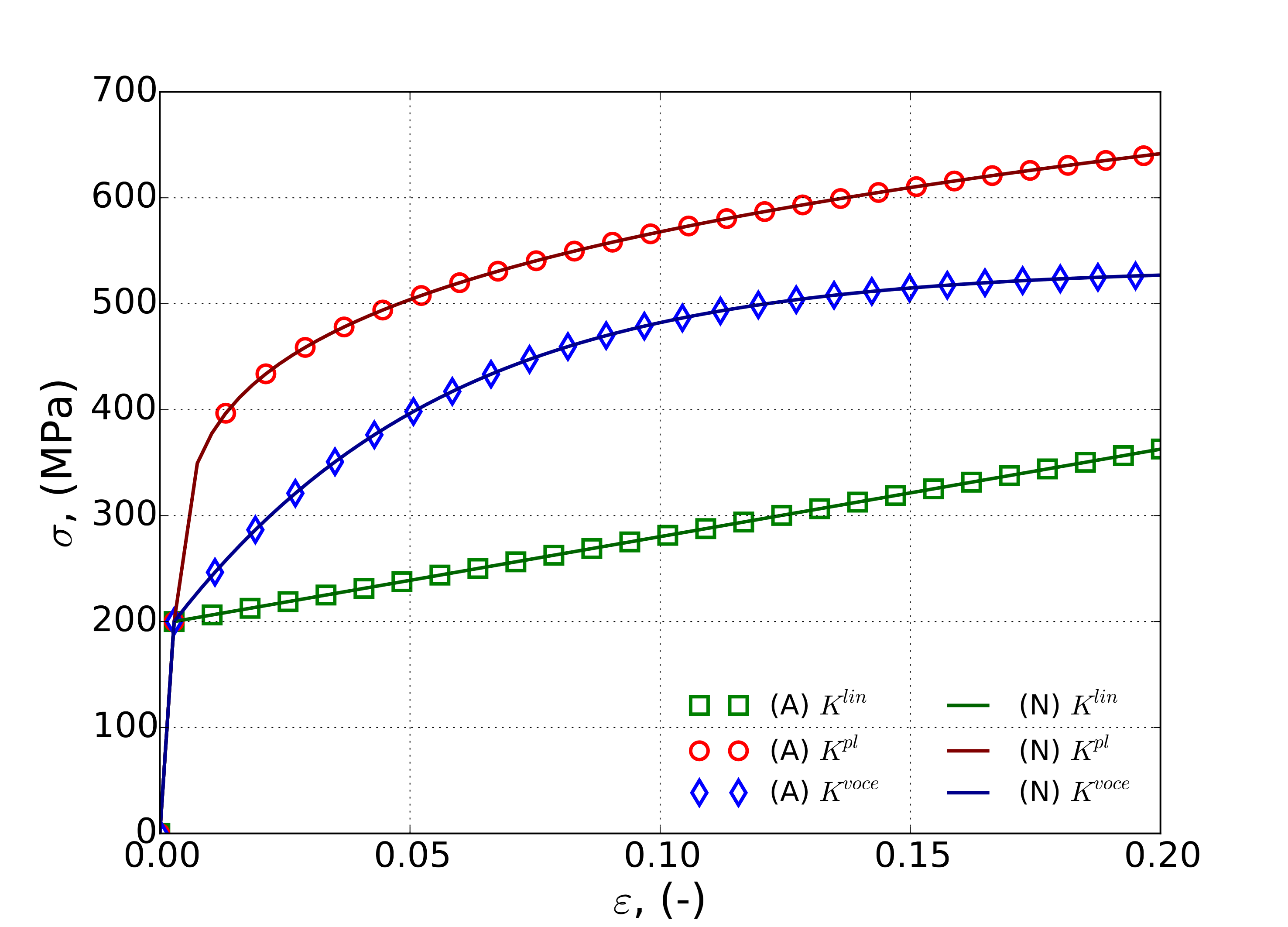
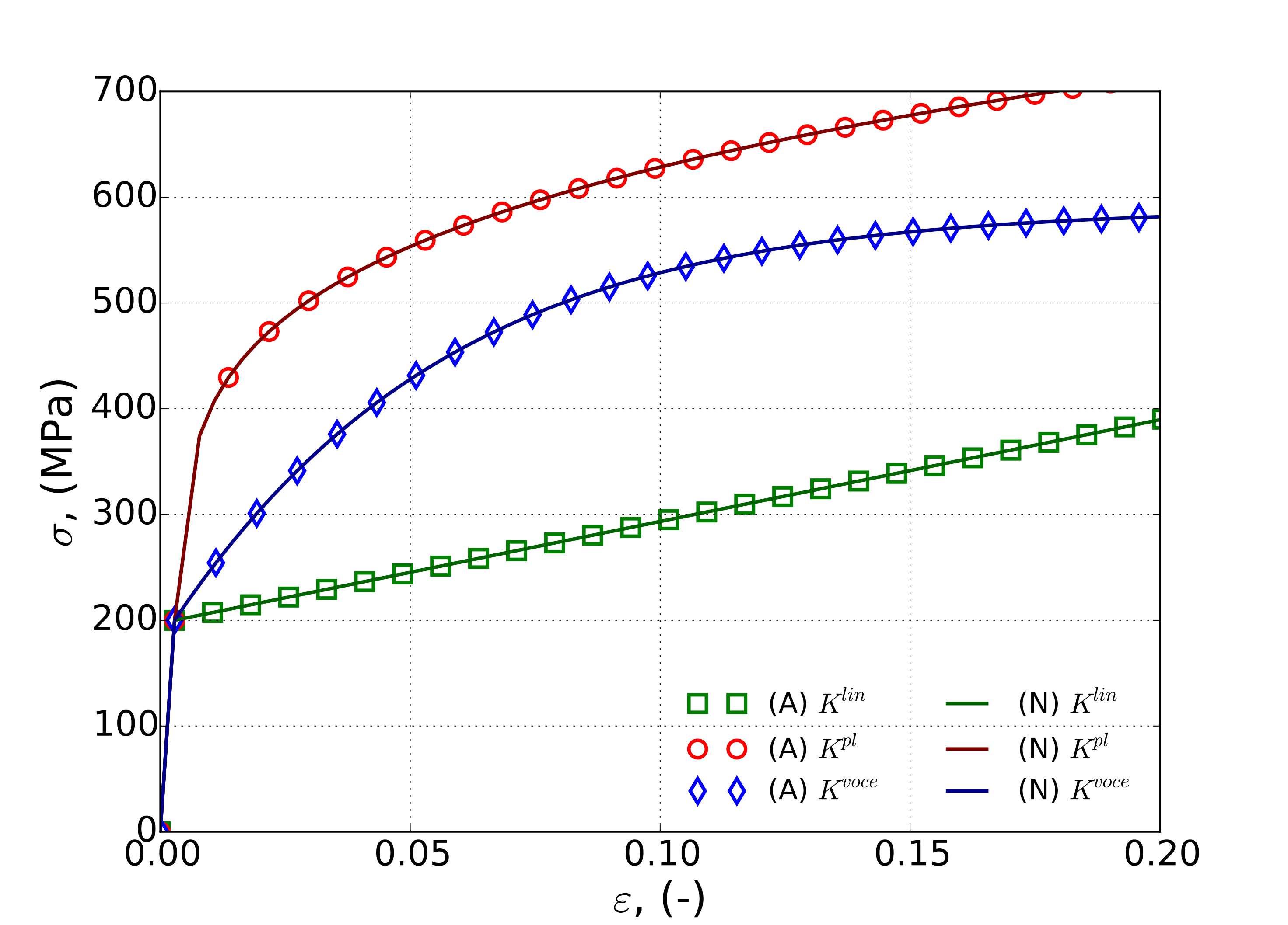
Fig. 4.92 Analytical and numerical constant equivalent plastic strain rate verification tests of the modular plane stress plasticity models with a uniaxial stress state and strain rates of (a) \(\dot{\varepsilon}^p=1\times 10^{-3}\)s\(^{-1}\) and (b) \(\dot{\varepsilon}^p=1\)s\(^{-1}\) with linear, power-law, and voce isotropic hardening and power-law breakdown rate-dependence. Solid lines are analytical and open symbols are from finite element calculations.

4.18.3.2. Balanced Biaxial

To assess performance of the model with multiple stress components, a constant equivalent plastic strain rate balanced biaxial test is considered. For this test, a stress-state (in the projected plane stress space) of

\[\begin{split}\underline{\sigma}\left(t\right)=\left[\begin{array}{c} \sigma\left(t\right) \\ -\sigma\left(t\right) \\ 0 \end{array}\right]\end{split}\]

is assumed. Note, such a loading is equivalent to a pure shear loading in a rotated frame of reference. As such, many of the pure shear results of Appendix A may be leveraged. To that end, if elasticity effects are included the total strain, \(\varepsilon\left(t\right)\), may be found to be

\[\varepsilon\left(t\right)=\frac{1}{\sqrt{3}}\frac{\sigma_y+\hat{\sigma}_hK\left(\dot{\bar{\varepsilon}}^p\left(t-t^{\text{el}}\right)\right)}{2\mu} + \frac{\sqrt{3}}{2}\dot{\bar{\varepsilon}}^p\left(t-t^{\text{el}}\right),\]

with \(t^{\text{el}}\) being the time at yield (elastic limit). To produce the desired stress state, the corrresponding displacements are \(u_1\left(t\right)=\exp\left(\varepsilon\left(t\right)\right)-1\) and \(u_2\left(t\right)=\exp\left(-\varepsilon\left(t\right)\right)-1\). Results of such tests and their corresponding analytical solutions are presented below in Fig. 4.93 with constant strain rates of \(\dot{\bar{\varepsilon}}^p=1\times 10^{-3}`s\ :math:`^{-1}\) (Fig. 4.93(a)) and \(\dot{\bar{\varepsilon}}^p=1\)s\(^{-1}\) (Fig. 4.93(b)).

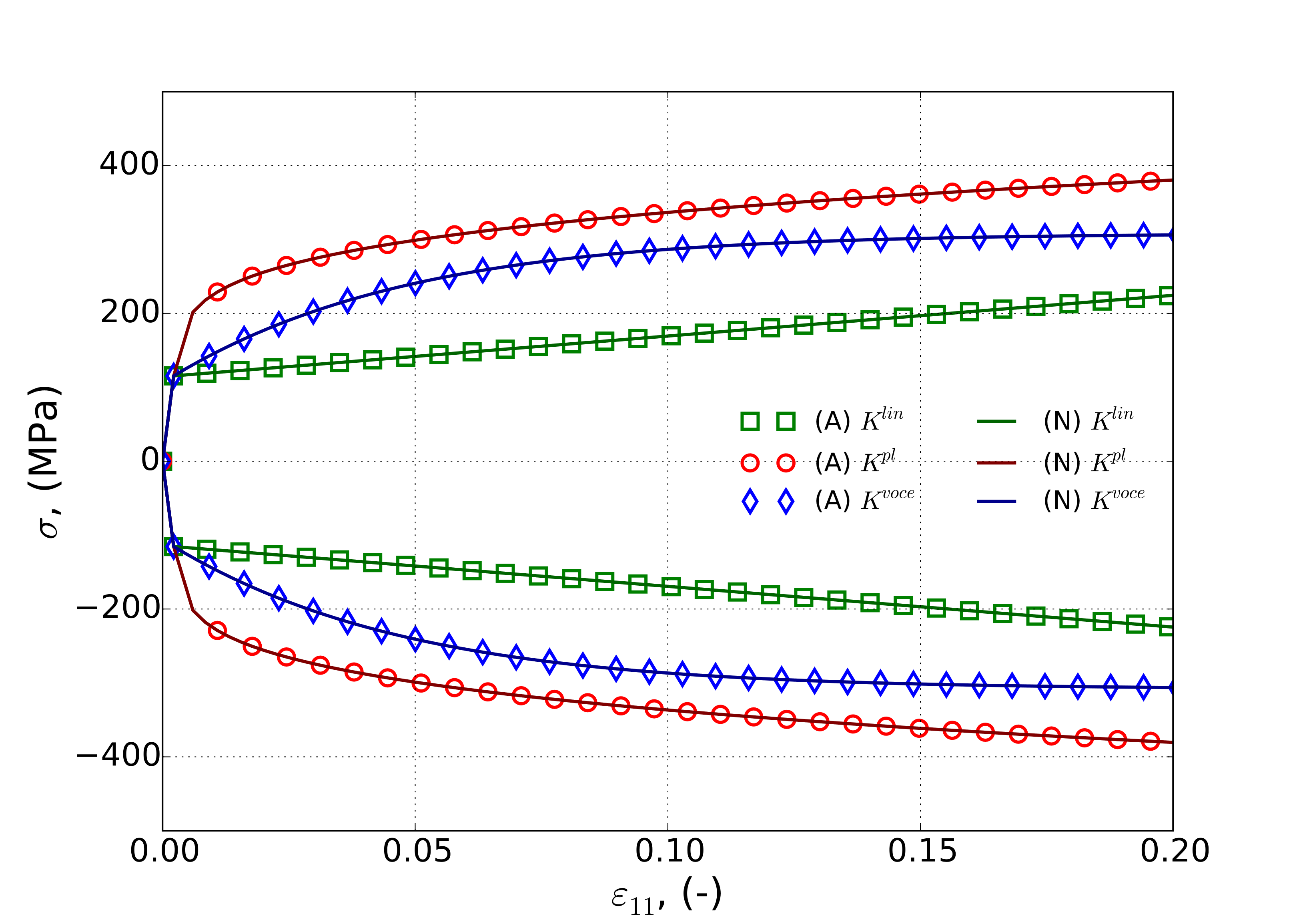
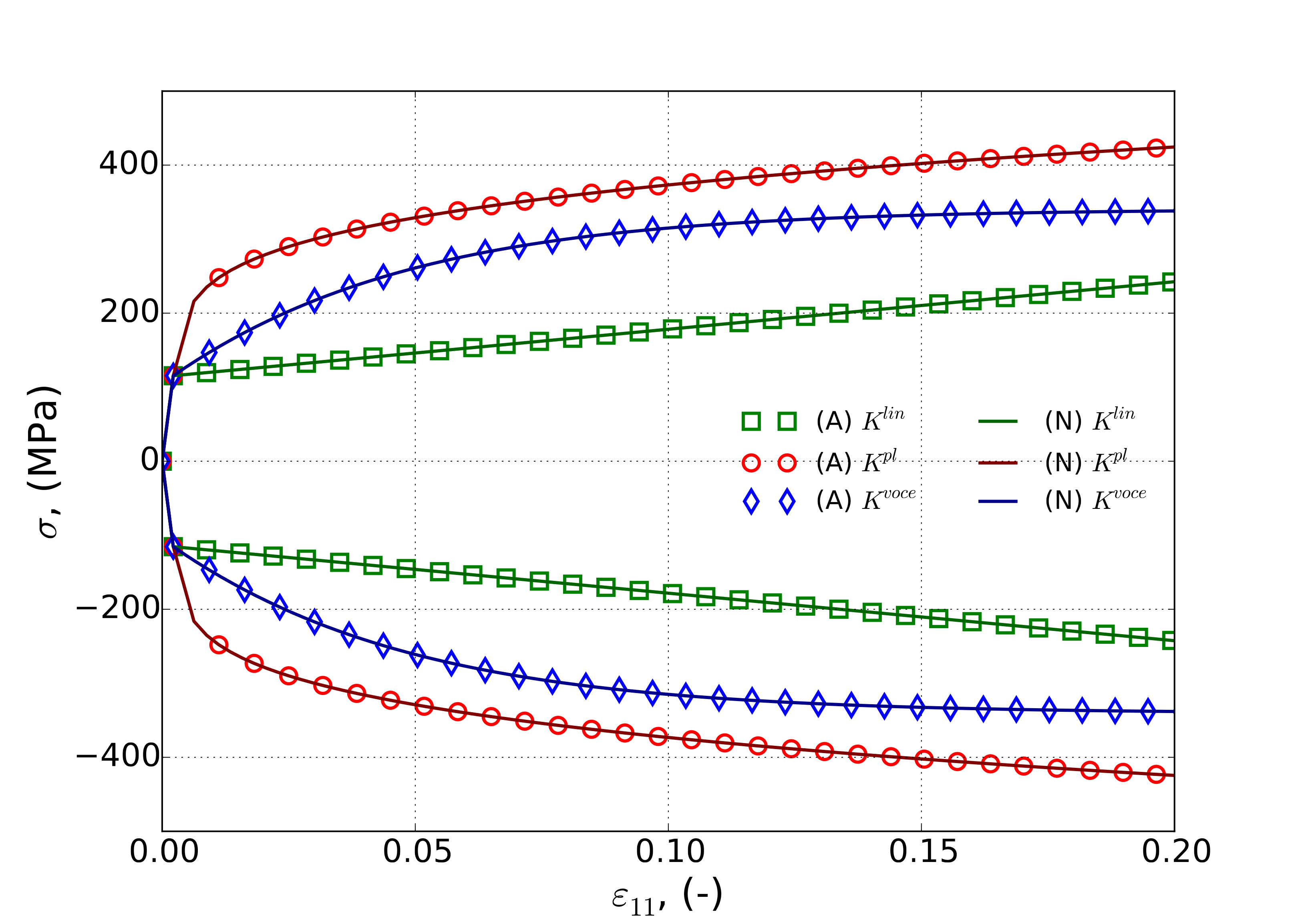
Fig. 4.93 Analytical and numerical constant equivalent plastic strain rate verification tests of the modular plane stress plasticity models with a balanced biaxial stress state and strain rates of (a) \(\dot{\varepsilon}^p=1\times 10^{-3}`s\ :math:`^{-1}\) and (b) \(\dot{\varepsilon}^p=1\)s\(^{-1}\) with linear, power-law, and voce isotropic hardening and power-law breakdown rate-dependence. Solid lines are analytical and open symbols are from finite element calculations. Positive valued stresses correspond to \(\sigma_{11}\) while negative values are \(\sigma_{22}\).

4.18.3.3. Biaxial Shear

As a final set of tests, the pure shear response is probed. To accomplish this loading, the previous balanced biaxial test is reconsidered with the geometry rotated 45\(^{\circ}\) about the out of plane direction producing a stress state of,

\[\begin{split}\underline{\sigma}\left(t\right)=\left[\begin{array}{c} 0 \\ 0 \\ \sigma_{xy}\left(t\right)\end{array}\right].\end{split}\]

The previous results from Section 4.18.3.2 regarding the solution for the balanced biaxial problem may again be used with \(\sigma_{xy}\left(t\right)=\sigma\left(t\right)\). Result for this case, both analytical and finite element, are given in Fig. 4.93 with constant applied strain rates of \(\dot{\bar{\varepsilon}}^p=1\times 10^{-3}`s\ :math:`^{-1}\) and \(\dot{\bar{\varepsilon}}^p=1\)s\(^{-1}\) in Fig. 4.94(a) and~:numref:fig-mpsp-verBiaxShear(b), respectively.

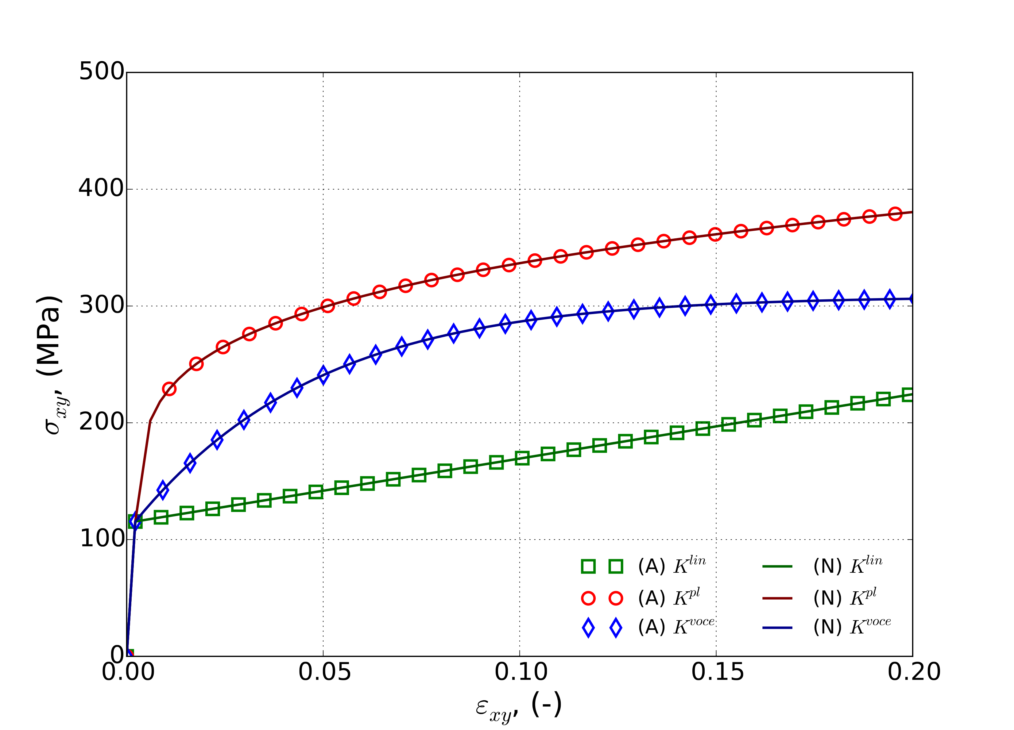
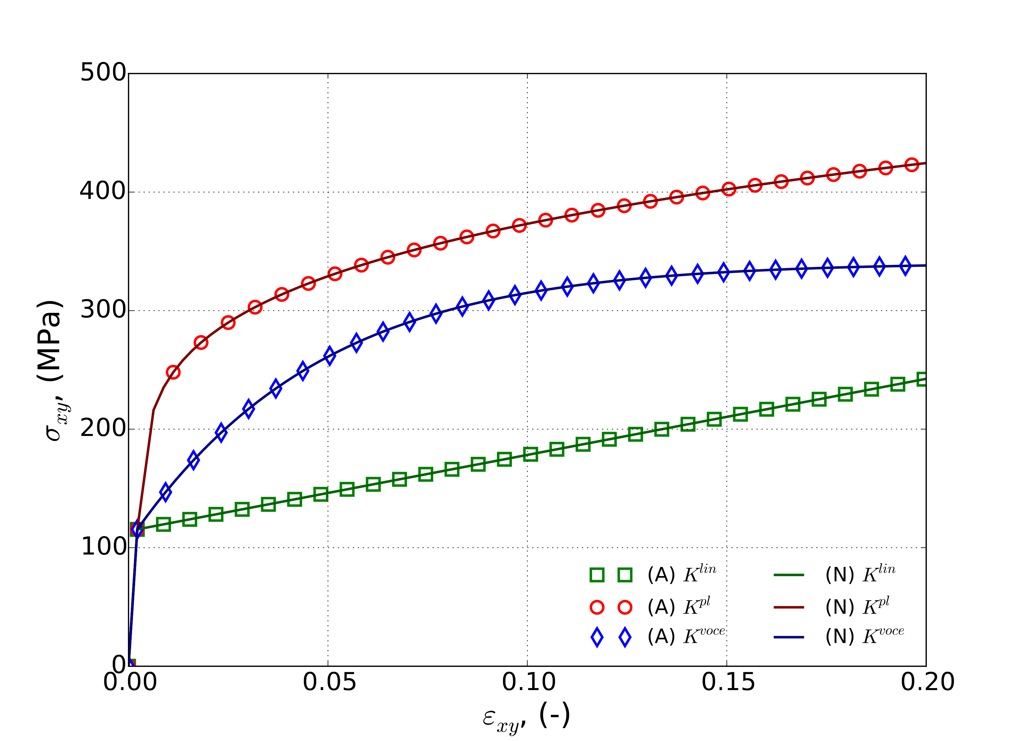
Fig. 4.94 Analytical and numerical constant equivalent plastic strain rate verification tests of the modular plane stress plasticity models with a pure shear stress state and strain rates of (a) \(\dot{\varepsilon}^p=1\times 10^{-3}`s\ :math:`^{-1}\) and (b) \(\dot{\varepsilon}^p=1`s\ :math:`^{-1}\) with linear, power-law, and voce isotropic hardening and power-law breakdown rate-dependence. Solid lines are analytical and open symbols are from finite element calculations.

4.18.4. User Guide

BEGIN PARAMETERS FOR MODEL MODULAR_PLANE_STRESS_PLASTICITY
   #
   # Elastic constants
   #
   YOUNGS MODULUS = <real>
   POISSONS RATIO = <real>
   SHEAR MODULUS  = <real>
   BULK MODULUS   = <real>
   LAMBDA         = <real>
   TWO MU         = <real>
   #
   YIELD STRESS   = <real>
   #

#
  #
  # Hardening model
  #
  HARDENING MODEL = LINEAR | POWER_LAW | VOCE | USER_DEFINED |
  FLOW_STRESS | DECOUPLED_FLOW_STRESS | JOHNSON_COOK |
  POWER_LAW_BREAKDOWN
  #
  # Linear hardening
  #
  HARDENING MODULUS = <real>
  #
  # Power-law hardening
  #
  HARDENING CONSTANT = <real>
  HARDENING EXPONENT = <real> (0.5)
  LUDERS STRAIN      = <real> (0.0)
  #
  # Voce hardening
  #
  HARDENING MODULUS       = <real>
  EXPONENTIAL COEFFICIENT = <real>
  #
  # Johnson-Cook hardening
  #
  HARDENING FUNCTION = <string>hardening_function_name
  RATE CONSTANT      = <real>
  REFERENCE RATE     = <real>
  #
  # Power law breakdown hardening
  #
  HARDENING FUNCTION = <string>hardening_function_name
  RATE COEFFICIENT   = <real>
  RATE EXPONENT      = <real>
  # User defined hardening
  #
  HARDENING FUNCTION = <string>hardening_function_name
  #

#
  #
  # Following Commands Pertain to Flow_Stress Hardening Model
  #
  #    -  Isotropic Hardening model
  #
  ISOTROPIC HARDENING MODEL = LINEAR | POWER_LAW | VOCE |
                              USER_DEFINED
  #
  # Specifications for Linear, Power-law, and Voce same as above
  #
  # User defined hardening
  #
  ISOTROPIC HARDENING FUNCTION = <string>iso_hardening_fun_name
  #
  #     - Rate dependence
  #
  RATE MULTIPLIER = JOHNSON_COOK | POWER_LAW_BREAKDOWN |
     RATE_INDEPENDENT (RATE_INDEPENDENT)
  #
  # Specifications for Johnson-Cook, Power-law-breakdown
  #     same as before EXCEPT no need to specify a
  #     hardening function
  #
  # User defined rate multiplier
  #
  RATE MULTIPLIER FUNCTION = <string> rate_mult_function_name
  #
  #
  # Following Commands Pertain to Decoupled_Flow_Stress Hardening Model
  #
  #    -  Isotropic Hardening model
  #
  ISOTROPIC HARDENING MODEL = LINEAR | POWER_LAW | VOCE | USER_DEFINED
  #
  # Specifications for Linear, Power-law, and Voce same as above
  #
  # User defined hardening
  #
  ISOTROPIC HARDENING FUNCTION = <string>isotropic_hardening_function_name
  #
  #     - Rate dependence
  #
  YIELD RATE MULTIPLIER = JOHNSON_COOK | POWER_LAW_BREAKDOWN |
              RATE_INDEPENDENT (RATE_INDEPENDENT)
  #
  # Specifications for Johnson-Cook, Power-law-breakdown same as before
  #     EXCEPT no need to specify a hardening function
  #     AND should be preceded by YIELD
  #
  #     As an example for Johnson-Cook yield rate dependence,
  #
  YIELD RATE CONSTANT  = <real>
  YIELD REFERENCE RATE = <real>
  #
  # User defined rate multiplier
  #
  YIELD RATE MULTIPLIER FUNCTION = <string>yield_rate_mult_function_name
  #
  HARDENING_RATE MULTIPLIER = JOHNSON_COOK | POWER_LAW_BREAKDOWN |
              RATE_INDEPENDENT (RATE_INDEPENDENT)
  #
  #     Syntax same as for yield parameters but with a HARDENING prefix
  #

END [PARAMETERS FOR MODEL MODULAR_PLANE_STRESS_PLASTICITY]

In the command blocks that define the Modular Plane Stress Plasticity model:

• The reference nominal yield stress, \(\bar{\sigma}\), is defined with the YIELD STRESS command line.

• The type of hardening law is defined with the HARDENING MODEL command line, other hardening commands then define the specific shape of that hardening curve.

• The hardening modulus for a linear hardening model is defined with the HARDENING MODULUS command line.

• The hardening constant for a power law hardening model is defined with the HARDENING CONSTANT command line.

• The hardening exponent for a power law hardening model is defined with the HARDENING EXPONENT command line.

• The Luders strain for a power law hardening model is defined with the LUDERS STRAIN command line.

• The hardening function for a user defined hardening model is defined with the HARDENING FUNCTION command line.

• The shape of the spline for the spline based hardening is defined by the CUBIC SPLINE TYPE, CARDINAL PARAMETER, KNOT EQPS, and KNOT STRESS command lines.

• The isotropic hardening model for the flow stress hardening model is defined with the ISOTROPIC HARDENING MODEL command line.

• The function name of a user-defined isotropic hardening model is defined via the ISOTROPIC HARDENING FUNCTION command line.

• The optional rate multiplier for the flow stress hardening model is defined with the RATE MULTIPLIER command line.

• The optional rate multiplier for the yield stress for the decoupled flow stress hardening model is defined with the YIELD RATE MULTIPLIER command line.

• The optional rate multiplier for the hardening for the decoupled flow stress hardening model is defined with the HARDENING RATE MULTIPLIER command line.

Output variables available for this model are listed in Table 4.27.

Table 4.27 State Variables for MODULAR PLANE STRESS PLASTICITY Model

Name	Description
RADIUS	yield surface radius in deviatoric \(\pi\)-plane, \(R\)
EQPS	equivalent plastic strain, \(\bar{\varepsilon}^{p}\)
EQDOT	equivalent plastic strain rate, \(\dot{\bar{\varepsilon}}^{p}\)
TENSILE_EQPS	tensile equivalent plastic strain, \(\bar{\varepsilon}^{p}_{t}\)

---

[1] (1,2,3,4,5,6)

J. C. Simo and R. L. Taylor. A return mapping algorithm for plane stress elastoplasticity. International Journal for Numerical Methods in Engineering, 22:649–670, 1986.

[2] (1,2,3,4)

J.C. Simo and T.J.R. Hughes. Computational Inelasticity. Springer-Verlag, New York, NY, 1998.

[3]

R. Hill. The Mathematical Theory of Plasticity. Oxford University Press, 1950.

[4]

J. Lemaitre and J.-L. Chaboche. Mechanics of Solid Materials. Cambridge University Press, 1990.

[5]

J. Lubliner. Plasticity Theory. Dover, 2008.

[6] (1,2,3)

G.R. Johnson and W.H. Cook. A constitutive model and data for metals subjected to large strains, high strain rates and high temperatures. In Proc. 7th. Int. Symp. on Ballistics, 541–547. The Hague, The Netherlands, 1983.

[7] (1,2,3)

G.R. Johnson and W.H. Cook. Fracture characteristics of three metals subjected to various strains, strain rates, temperatures and pressures. Engineering Fracture Mechanics, 21(1):31–48, 1985.

[8]

H. J. Frost and M. F. Ashby. Deformation Mechanism Maps: the Plasticity and Creep of Metals and Ceramics. Pergamon Press, 1982.

[9]

A.A. Brown and D.J. Bammann. Validation of a model for static and dynamic recrystallization in metals. International Journal of Plasticity, 32–33:17–35, 2012.

[10] (1,2)

W. M. Scherzinger. A return mapping algorithm for isotropic and anisotropic plasticity models using a line search method. Computer Methods in Applied Mechanics and Engineering, 317:526–553, 2017.