4.12. Johnson-Cook Model

4.12.1. Theory

The Johnson-Cook model [[1], [2]] is an isotropic, hypoelastic plasticity model. Unlike the previously discussed models, the Johnson-Cook formulation is rate-dependent and as such is often considered for high-rate, finite strain simulations like those for impact. The viscoplastic response is phenomenological in that the form of the model is not derived from any physical mechanisms like other viscoplastic models, e.g. Zerilli-Armstrong [[3]], Steinberg-Guinan-Lund [[4], [5]], BCJ [[6]], and the MTS model [[7], [8]] to name a few. Like most other rate-dependent models, the current formulation utilizes an effective plastic strain rate, \(\dot{\bar{\varepsilon}}^{p}\), to capture rate dependence.

As with other hypoelastic plasticity models, an additive decomposition of of the total rate of deformation such that,

\[D_{ij}=D^{\text{e}}_{ij}+D^{\text{p}}_{ij},\]

is used such that an objective stress rate of the form,

\[\stackrel{\circ}{\sigma}_{ij}=\mathbb{C}_{ijkl}D_{kl}^{\text{e}},\]

with \(\mathbb{C}_{ijkl}\) being the fourth-order, isotropic elasticity tensor, may be used.

With respect to the yield behavior, the Johnson-Cook model incorporates both strain rate and temperature, \(\theta\), dependence. This leads to a yield function of the form,

\[f\left(\sigma_{ij},\bar{\varepsilon}^p,\dot{\bar{\varepsilon}}^p,\theta\right)=\phi\left(\sigma_{ij}\right)-\bar{\sigma}\left(\bar{\varepsilon}^p,\dot{\bar{\varepsilon}}^p,\theta\right),\]

in which \(\phi\left(\sigma_{ij}\right)\) is the effective stress – the von Mises effective stress is used – and \(\bar{\sigma}\) is the isotropic hardening function. Incorporating the temperature and rate dependency, the hardening function is written as,

(4.38)\[\bar{\sigma}\left(\bar{\varepsilon}^p,\dot{\bar{\varepsilon}}^p,\theta\right) = \left[ A + B \left(\bar{\varepsilon}^p\right)^{N} \right] \left[ 1 + C \left<\ln \dot{\bar{\varepsilon}}^{p*}\right> \right] \left[ 1 - \theta^{*\,M} \right]\]

where \(\bar{\varepsilon}^p\) is the equivalent plastic strain, \(\dot{\bar{\varepsilon}}^{p*} = \dot{\bar{\varepsilon}}^p/\dot{\bar{\varepsilon}}_{0}\) is a dimensionless plastic strain rate, and \(\theta^{*}\) is the homologous temperature. The quantities \(A\), \(B\), \(C\), \(\dot{\bar{\varepsilon}}_{0}\), \(N\), and \(M\) are material parameters. The Macaulay brackets in eqref{jc:theory:eqn:flowStress} ensure that \(\bar{\sigma}\) is equal to the static flow stress \(\bar{\sigma}_{\text{s}} = \left[ A + B \left(\bar{\varepsilon}^p\right)^{N} \right]\left[ 1 - \theta^{*\,M} \right]\) when \(\dot{\bar{\varepsilon}}^p<\dot{\bar{\varepsilon}}_{0}\). The homologous temperature is defined as,

(4.39)\[\theta^{*}=\frac{\theta-\theta_{\text{ref}}}{\theta_{\text{melt}}-\theta_{\text{ref}}},\]

with \(\theta,~\theta_{\text{ref}}\), and \(\theta_{\text{melt}}\) being the current, reference, and melt temperatures. Note, the temperature used internal to the Johnson-Cook model is NOT the standard prescribed “temperature” field. Instead, the material temperature is initialized by a model input as \(\theta_0\). By assuming adiabatic thermal conditions, subsequent plastic work raises the material temperature via,

\[\Delta\theta=\frac{\beta}{\rho C_{v}}\bar{\sigma}\dot{\bar{\varepsilon}}^p,\]

where \(\rho\) is the materials density, \(C_{v}\) is the specific heat, and \(\beta\) (\(0\leq\beta\leq 1\)) is the fraction of plastic work that is converted to heat.

The Johnson-Cook model also has a failure criterion. The Johnson-Cook damage model [[2]] has a failure strain that is given by:

\[\varepsilon^f=\left(D_1+D_2\exp\left(D_3\eta\right)\right)\left(1+D_4\ln\dot{\bar{\varepsilon}}^{p*}\right)\left(1+D_5\theta^{*}\right)\]

with \(D_1,~D_2,~D_3,~D_4,\) and \(D_5\) being material parameters and \(\eta\) is the triaxiality (\(\eta=\left(1/3\right)\sigma_{kk}/\bar{\sigma}_{vM}\)). The damage in the model is accumulated over time using:

(4.40)\[D=\int_0^t\frac{\dot{\bar{\varepsilon}}^{p}}{\varepsilon^f}dt.\]

When \(D=1\), the material has failed. For the default behavior of the Johnson-Cook model, the fracture behavior is not active.

4.12.2. Implementation

The implementation of the Johnson-Cook model requires the effective strain rate to be used for calculating the rate effects on yield. This is done through a predictor-corrector return mapping algorithm. In what follows the temperature dependence is not included; this will be addressed later.

The initial response is assumed to be elastic and a trial stress state is calculated

\[T_{ij}^{\text{tr}} = T_{ij}^{n} + \mathbb{C}_{ijkl}\,\Delta\,t d_{kl}\]

Since the plastic response is independent of pressure we can use the deviatoric stress

\[\begin{split}s_{ij} = T_{ij} - \frac{1}{3}\delta_{ij}T_{kk} \\ s_{ij}^{\text{tr}} = s_{ij}^{n} + 2\mu\,\Delta\,t d_{ij}^{\prime},\end{split}\]

with \(d_{ij}^{\prime}\) being the total deviatoric rate of deformation – \(d_{ij}^{\prime}=d_{ij}-\left(1/3\right)\delta_{ij}d_{kk}\).

If this gives a von Mises stress that is greater then the effective stress, i.e.

\[\phi^{\text{tr}} = \sqrt{\frac{3}{2} s_{ij}^{\text{tr}}s_{ij}^{\text{tr}}} > A + B \left(\bar{\varepsilon}^{p\left(n\right)}\right)^{N},\]

then plastic deformation occurs and we solve the following nonlinear equation for \(\dot{\bar{\varepsilon}}^p\),

(4.41)\[\left[ A + B \left( \bar{\varepsilon}_{p\left(n\right)} + \Delta t \dot{\bar{\varepsilon}}^p \right)^{N} \right] \left[ 1 + C \ln \left( \max \left( 1, \dot{\bar{\varepsilon}}^p / \dot{\bar{\varepsilon}}_{0} \right) \right) \right] = \phi^{\text{tr}} - 3\mu \Delta t \dot{\bar{\varepsilon}}^p.\]

This simple equation comes from the radial return algorithm

\[s_{ij}^{n+1} = s_{ij}^{\text{tr}} - 3\mu \, \Delta t \, \dot{\bar{\varepsilon}}^p \, \frac{s_{ij}^{\text{tr}}}{\phi^{\text{tr}}} \;\;\; \rightarrow \;\;\; s_{ij}^{n+1} = \left( \phi^{\text{tr}} - 3\mu \, \Delta t \, \dot{\bar{\varepsilon}}^p \right) \frac{s_{ij}^{\text{tr}}}{\phi^{\text{tr}}}\]

Taking the inner product of both sides gives (4.41).

4.12.3. Verification

The Johnson-Cook model is verified through a series of uniaxial stress and pure shear tests. Given the emphasis on the strain-rate and temperature dependent nature of the model a series of these tests are performed at different loading conditions. The material properties and model parameters used for these tests are given in Table 4.14 and come from the work of Corona and Orient [[9]]. Note, in this case a modified reference plastic strain rate is used (\(\dot{\bar{\varepsilon}}_0=1\times 10^{-4} \text{s}^{-1}\)) as the one reported in [[9]] was selected based on calibration conditions. Here the value is selected to better investigate and highlight strain rate dependency.

Table 4.14 The material properties and model parameters of the Johnson-Cook model used for verification testing

\(E\)	71.7 GPa	\(\nu\)	0.33
\(A\)	217 MPa	\(B\)	405 MPa
\(C\)	0.0075	\(\dot{\bar{\varepsilon}}_0\)	1 \(\times 10^{-4}\) s\(^{-1}\)
\(\theta_{\text{ref}}\)	293 K	\(\theta_{\text{melt}}\)	750 K
\(N\)	0.41	\(M\)	1.1
\(\rho\)	2810 kg/m \(^3\)	\(C_v\)	960 J/(kg-K)
\(D_1\)	0.015	\(D_2\)	0.24
\(D_3\)	-1.5	\(D_4\)	-0.039
\(D_5\)	8.0

4.12.3.1. Uniaxial Stress

To determine a (semi)-analytical expression of the Johnson-Cook model, the equivalency of plastic work for uniaxial loading is recalled such that,

(4.42)\[\bar{\sigma}\dot{\bar{\varepsilon}}^p=\sigma\left(\dot{\varepsilon}-\dot{\varepsilon}^{\text{e}}\right),\]

with \(\sigma\), \(\dot{\varepsilon}\), and \(\dot{\varepsilon}^{\text{e}}\) being the uniaxial stress, total strain rate, and elastic strain rate, respectively. Assuming \(\dot{\bar{\varepsilon}}^{p}\ge\dot{\bar{\varepsilon}}_0\), and noting that \(\dot{\varepsilon}^{p}=\dot{\varepsilon}-\dot{\varepsilon}^{\text{e}}\), the expression for the flow stress (4.38), the definition of the homologous temperature (4.39), and the dimensionless strain rate, the plastic work expression (4.42) may be rearranged as

(4.43)\[\dot{\bar{\varepsilon}}^p=\dot{\bar{\varepsilon}}_0\exp\left[\frac{\sigma}{C\left[A+B\left(\bar{\varepsilon}^p\right)^N\right]\left[1-\theta^{*M}\right]}-\frac{1}{C}\right].\]

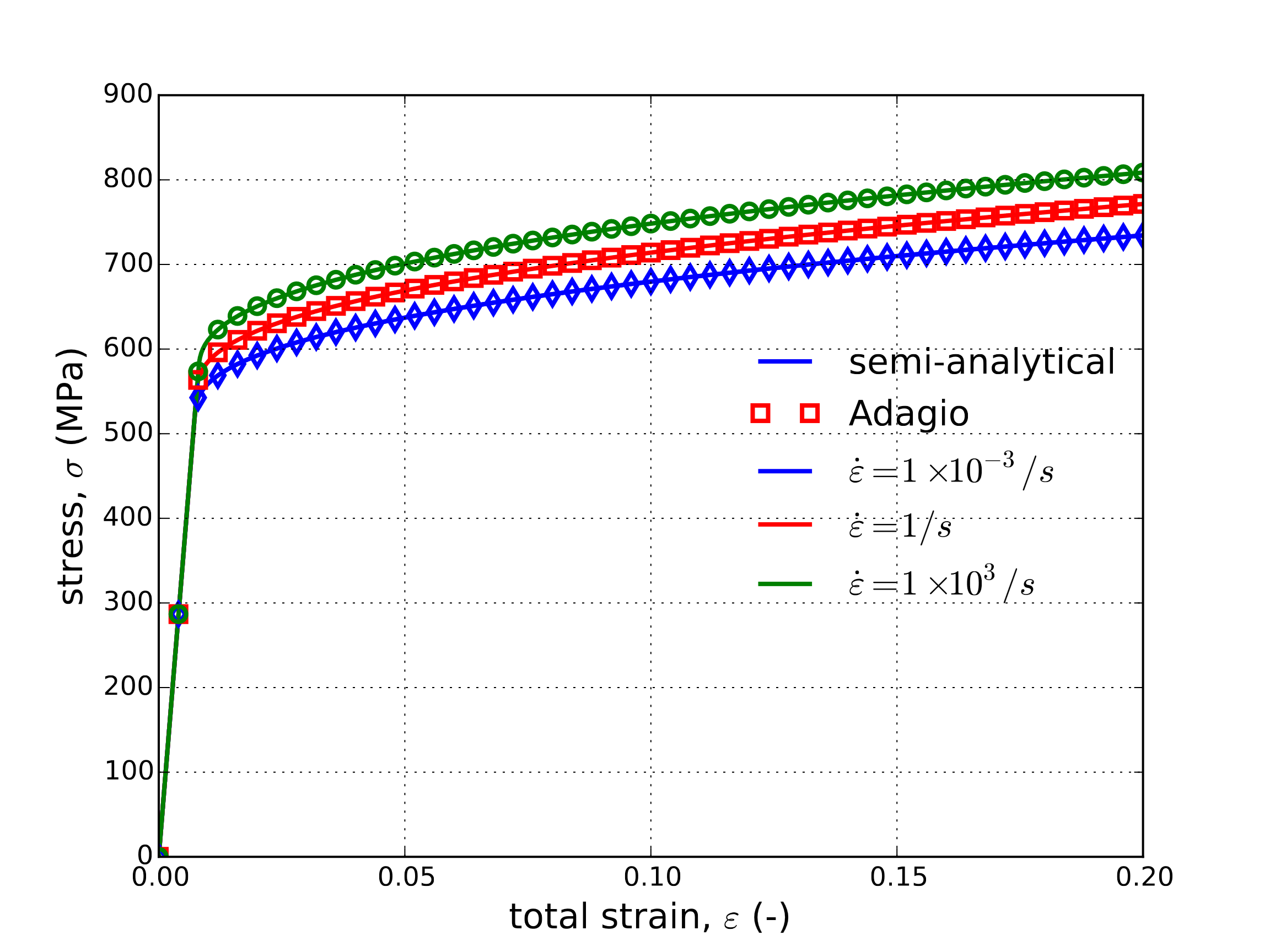
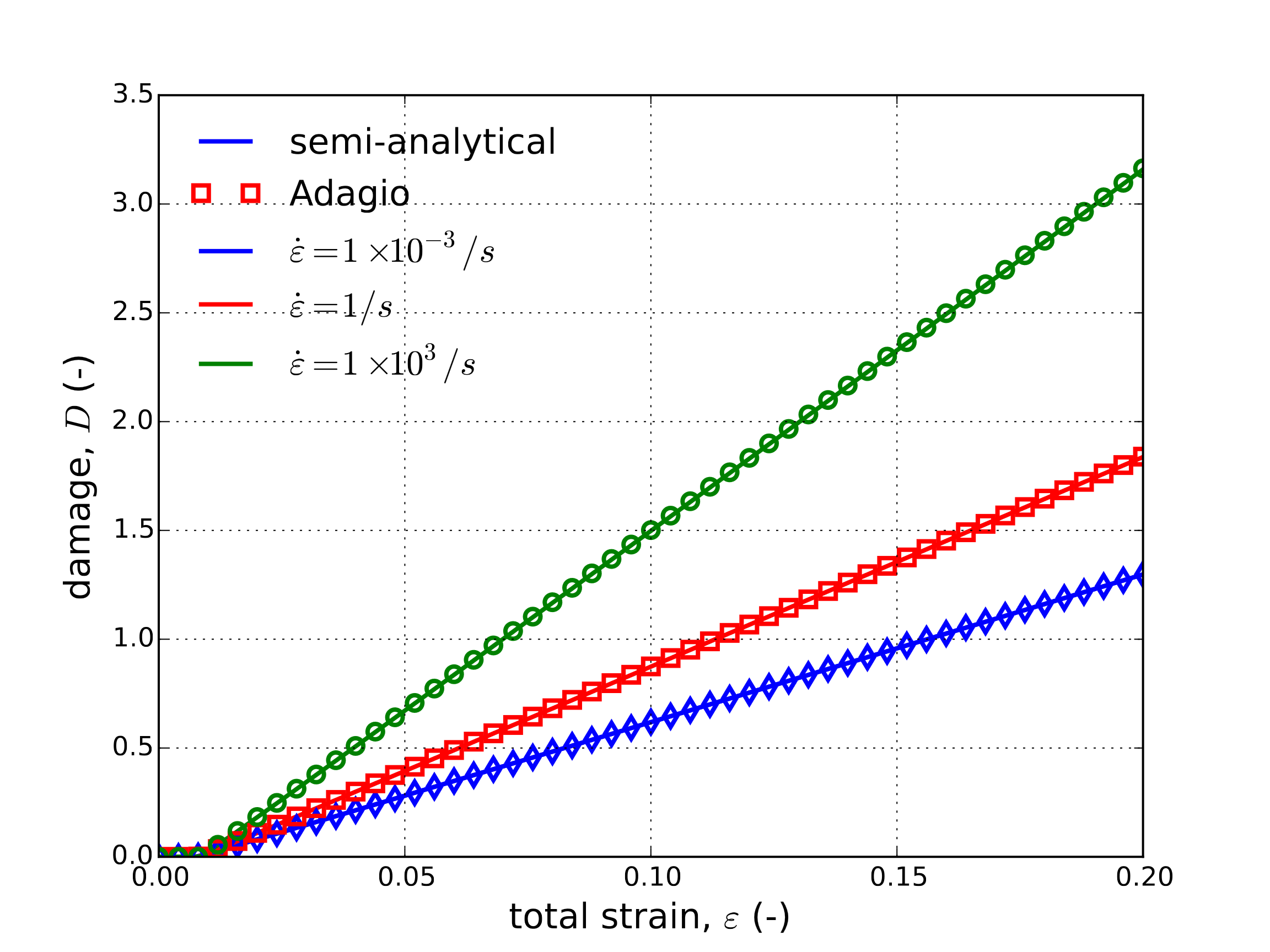
Given the implicit nature (in terms of effective plastic strain) of eqref{jc:ver:uni:eqps}, a semi-analytical approach is used to evaluate the Johnson-Cook model. Specifically, a simple forward Euler integration scheme is adopted to solve eqref{jc:ver:uni:eqps} and then update the remaining state variables. Using such an approach, Fig. 4.33 presents the stress-strain and corresponding damage evolution of the Johnson-Cook determined at three strain rates. A constant total logarithmic strain rate is applied by utilizing an applied displacement of the form,

\[u_i\left(t\right)=\left(\text{e}^{\omega t}-1\right)\delta_{i1},\]

where \(\omega\) is the considered strain rate. Here rates corresponding to a slow quasistatic (\(\omega=1\times 10^{-3}\text{s}^{-1}\)), medium (\(\omega=1\text{s}^{-1}\)), and high rate (\(\omega=1\times 10^3\text{s}^{-1}\)) loading are considered to explore a variety of regimes. Temperature effects are not addressed in Fig. 4.33 (\(\beta=0\)) to first investigate the purely mechanical response. The damage evolution is evaluated by simply integrating expression eqref{jc:theory:eqn:dam} and noting that for a uniaxial loading \(\eta=1/3\). In this case, as the constitutive behavior is being probed the material does not degrade when \(D\geq 1\).

Stress-strain

Damage

Fig. 4.33 Semi-analytical and numerical (a) stress-strain and (b) damage evolutions of the Johnson-Cook model subjected to a uniaxial loading at three different applied strain rates. In these results, \(\beta=0\).

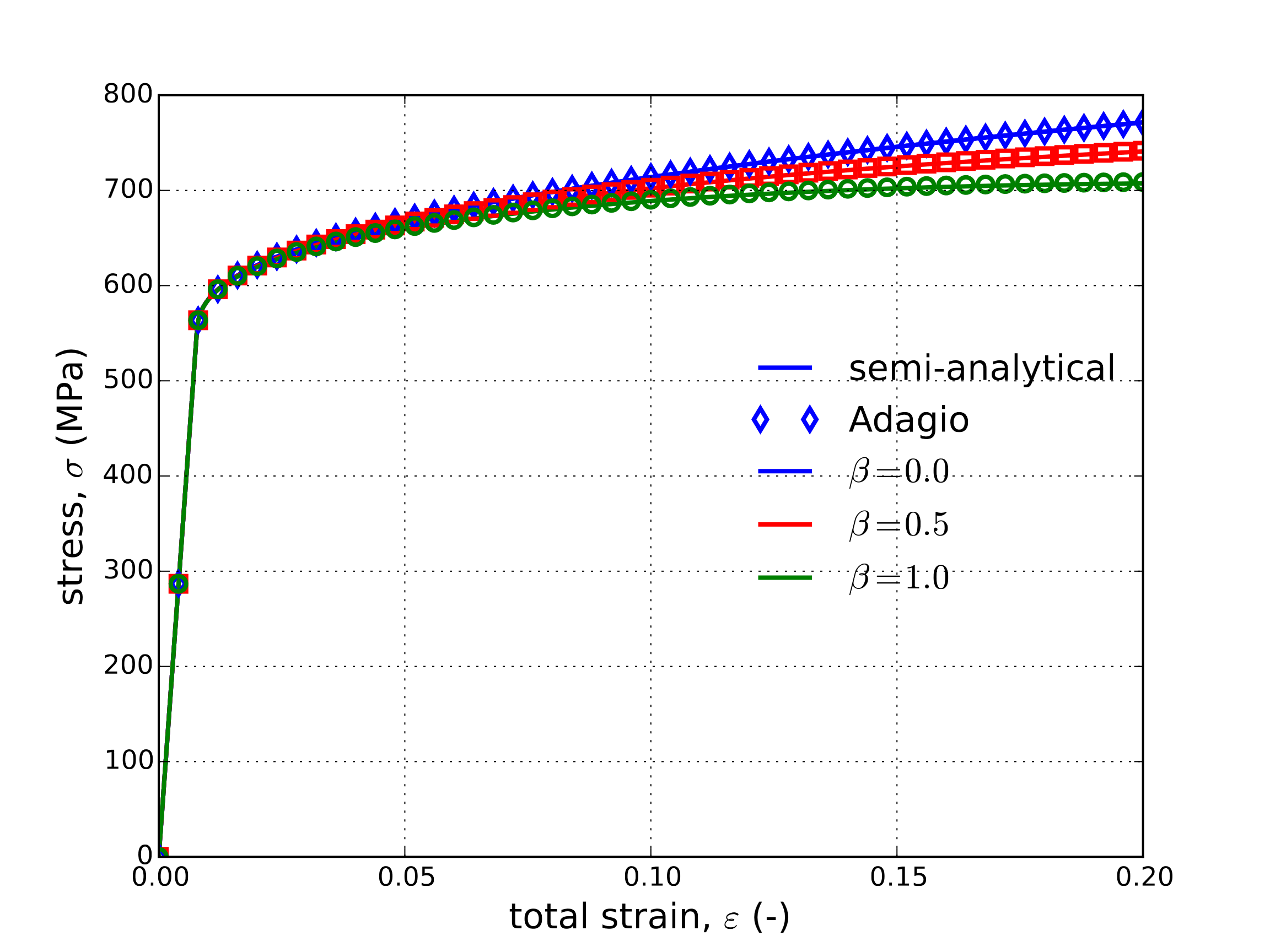
From the results of Fig. 4.33 clear agreement is observed between the numerical and semi-analytical response verifying the model behavior in a variety of conditions. Next, to explore the thermomechanical coupling, three different plastic work conversion ratios (\(\beta=0.00,~0.50\) and \(1.0\)) are considered for the medium strain rate (\(\omega = 1\text{s}^{-1}\)). The stress, damage, and temperature evolutions are all presented in Fig. 4.34 as a function of axial strains.

Stress-strain

Damage

Temperature

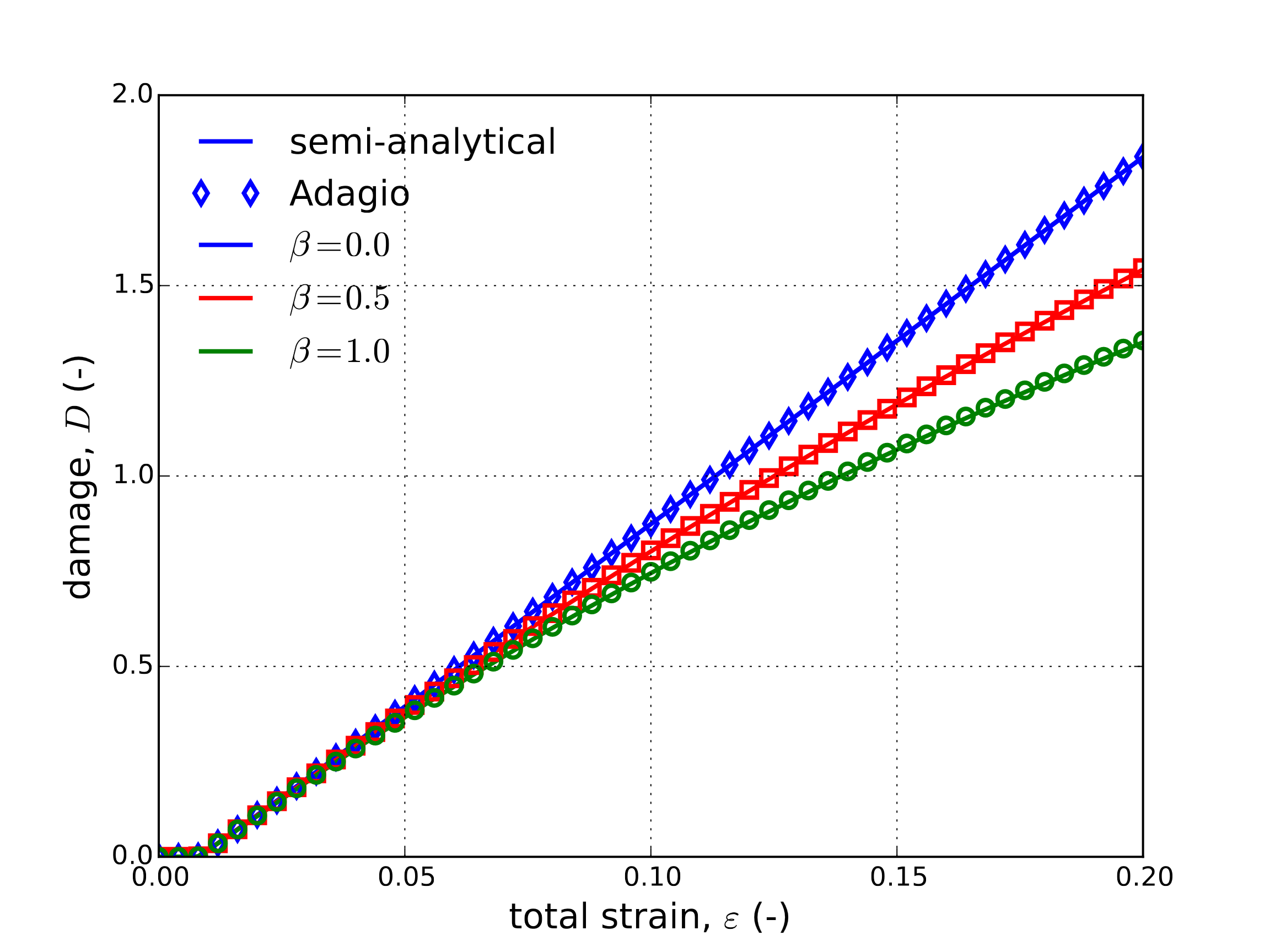
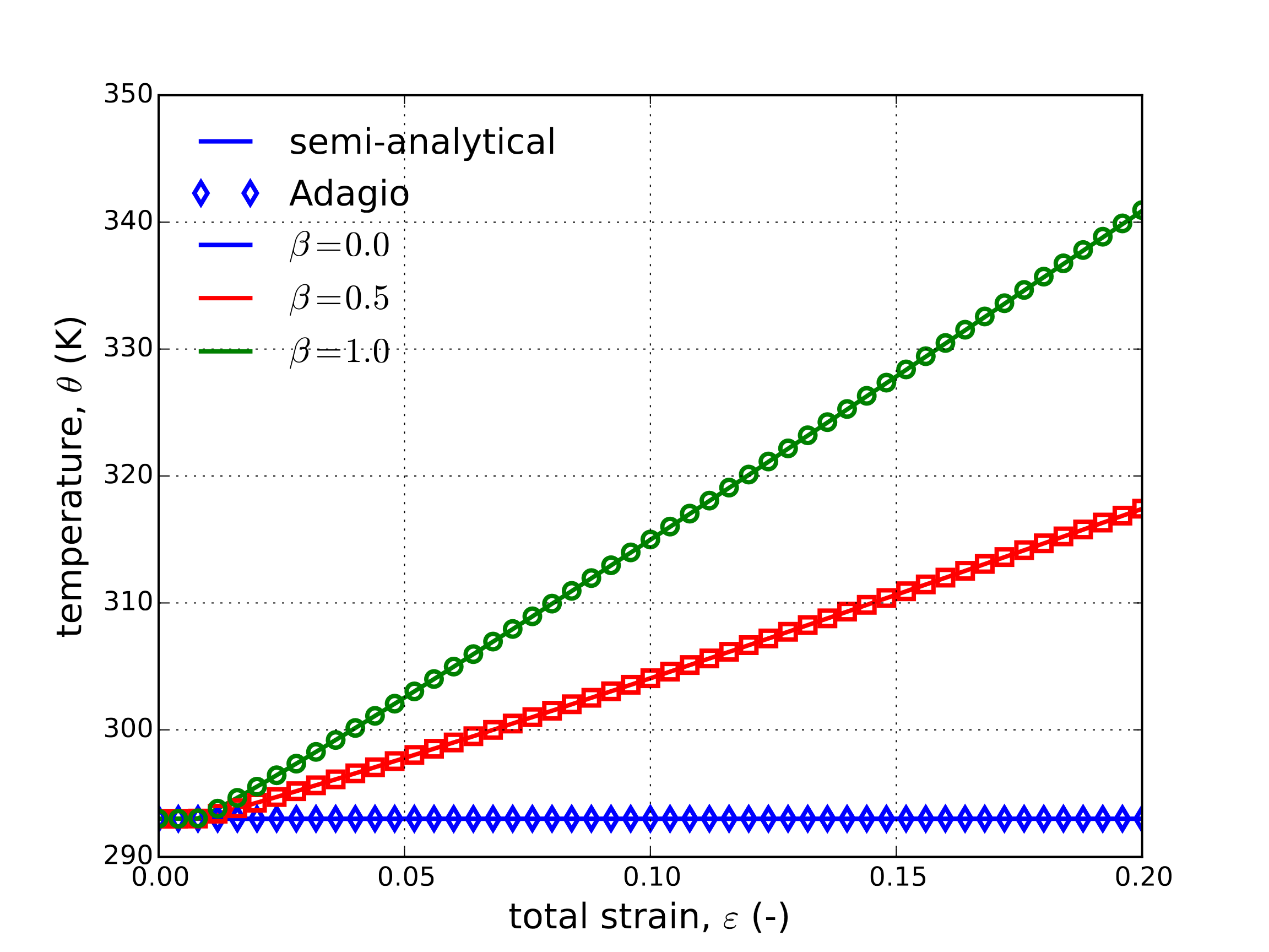
Fig. 4.34 Semi-analytical and numerical (a) stress-strain (b) damage and (c) temperature evolutions of the Johnson-Cook model subjected to a uniaxial loading with three different plastic work conversion ratios, \(\beta\). The strain rate for all three cases is \(\dot{\varepsilon}=1\text{s}^{-1}\).

From Fig. 4.34 the influence of the thermomechanical coupling may be clearly observed. For instance, a roughly 50 K increase in material temperature over the loading range may be seen in the \(\beta=1\) case leading to a roughly 25% decrease in the damage metric and approximately 10% drop in final stress. Additionally, clear agreement between the semi-analytical and numerical responses providing additional verification of the coupled capabilities of the model.

4.12.3.2. Pure Shear

For the pure shear case, a loading like that described in Appendix A is utilized. Specifically, displacements producing a deformation gradient of,

\[F_{ij}=\frac{1}{2}\left(\lambda+\lambda^{-1}\right)\left(\delta_{i1}\delta_{j1}+\delta_{i2}\delta_{j2}\right)+\frac{1}{2}\left(\lambda-\lambda^{-1}\right)\left(\delta_{i1}\delta_{j2}+\delta_{i2}\delta_{j1}\right)+\delta_{i3}\delta_{j3},\]

are considered with \(\lambda=\lambda\left(t\right)=\text{e}^{\omega t}\). This loading leads to a logarithmic shear strain rate of \(\dot{\varepsilon}_{12}=\omega\) that is constant in time enabling the study of strain rate effects.

In the shear stress case, the plastic work equivalency is written as,

\[\bar{\sigma}\dot{\bar{\varepsilon}}^p=2\sigma_{12}\dot{\varepsilon}^p_{12}.\]

Like the uniaxial stress case, the definition of the effective stress may be used with the fact that \(\dot{\varepsilon}^p_{12}=\frac{\sqrt{3}}{2}\dot{\bar{\varepsilon}}^p\) to find the following form of the effective plastic strain rate when \(\dot{\bar{\varepsilon}}^{\text{p}}>\dot{\bar{\varepsilon}}_0\),

\[\dot{\bar{\varepsilon}}^p=\dot{\bar{\varepsilon}}_0\exp\left[\frac{\sqrt{3}\sigma_{12}}{C\left[A+B\left(\bar{\varepsilon}^p\right)^N\right]\left[1-\theta^{*M}\right]}-\frac{1}{C}\right].\]

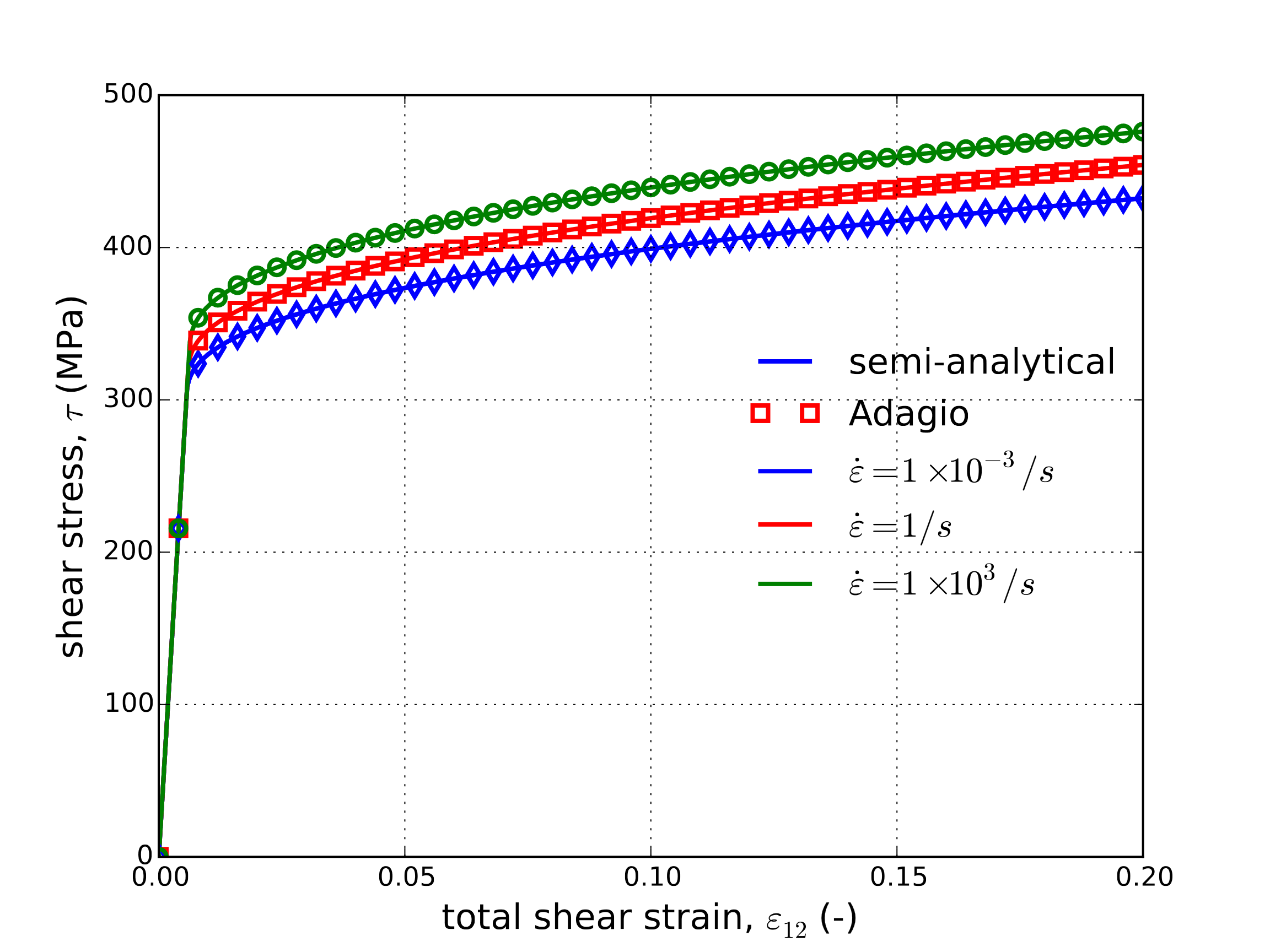
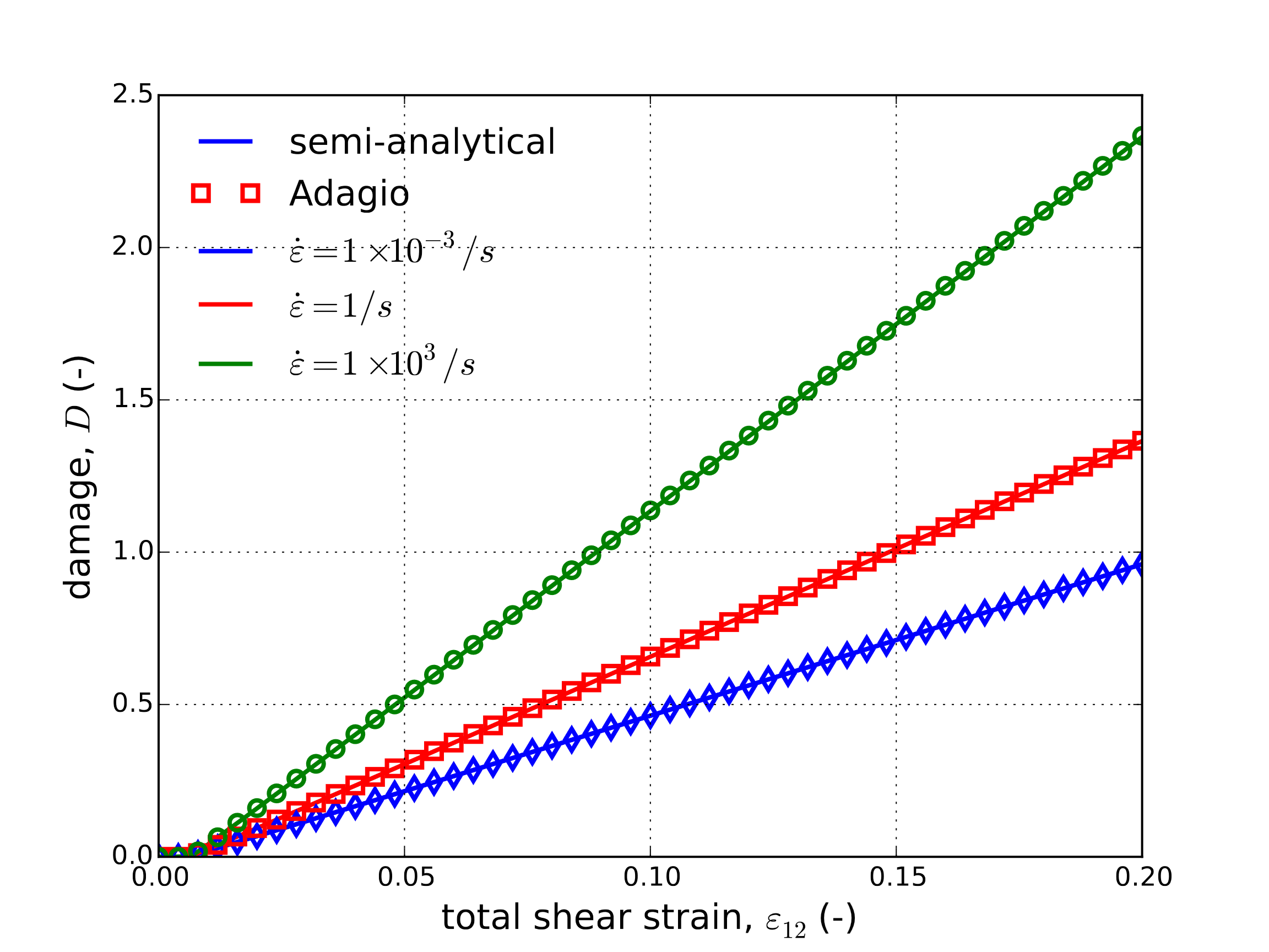
A simple forward Euler scheme is then used to integrate the model at three different strain rates – \(\omega=.001\text{s}^{-1}\), \(1\text{s}^{-1}\) and \(1000\text{s}^{-1}\). The stress-strain and damage evolution responses of these cases are presented in Fig. 4.35 for the purely mechanical case (\(\beta=0\)). With respect to the damage evolution, it is noted that for pure shear responses \(\eta=0\).

Stress-strain

Damage

Fig. 4.35 Semi-analytical and numerical (a) stress-strain and (b) damage evolutions of the Johnson-Cook model subjected to a pure shear loading at three different applied strain rates. In these results, \(\beta=0\).

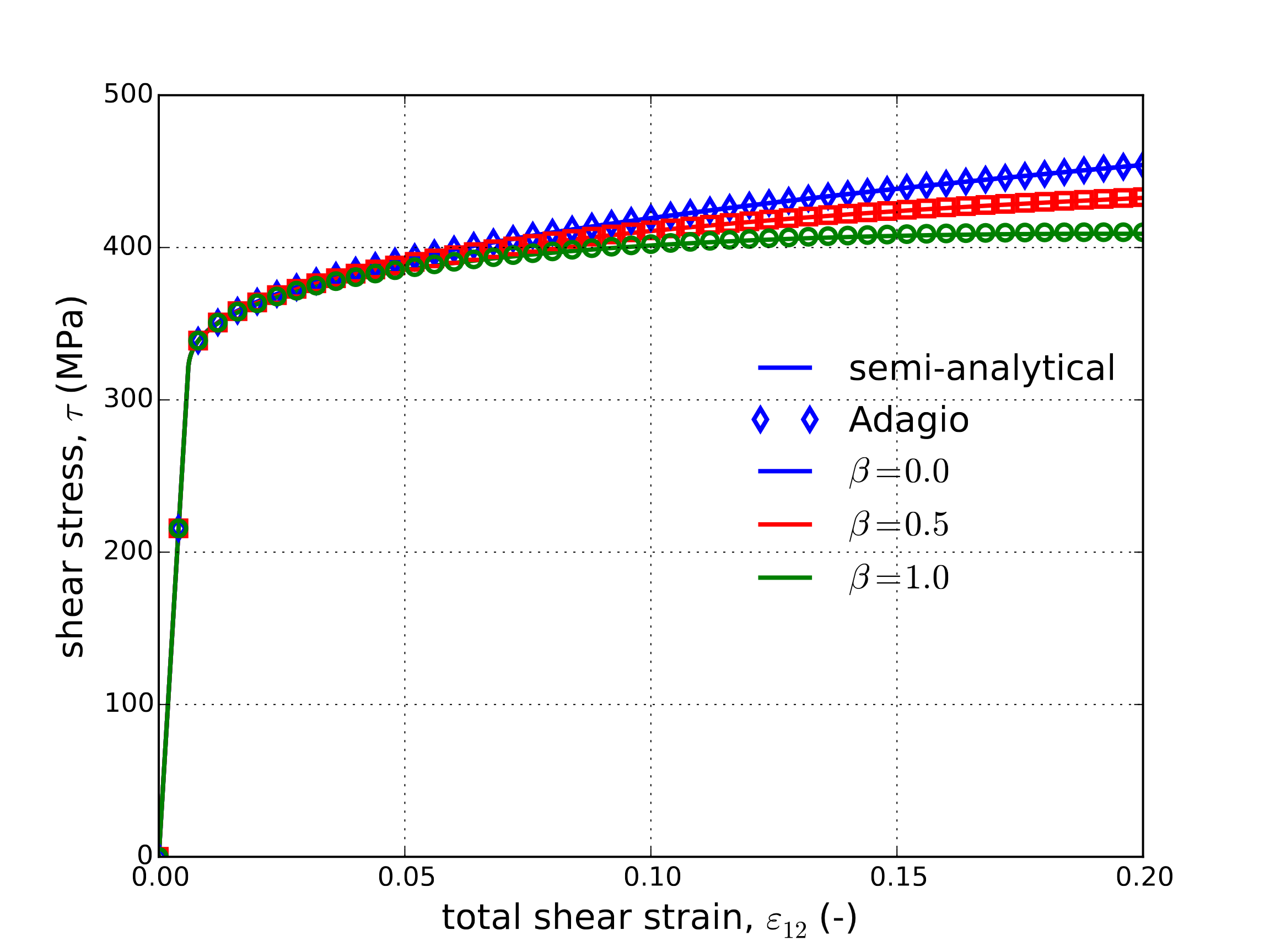
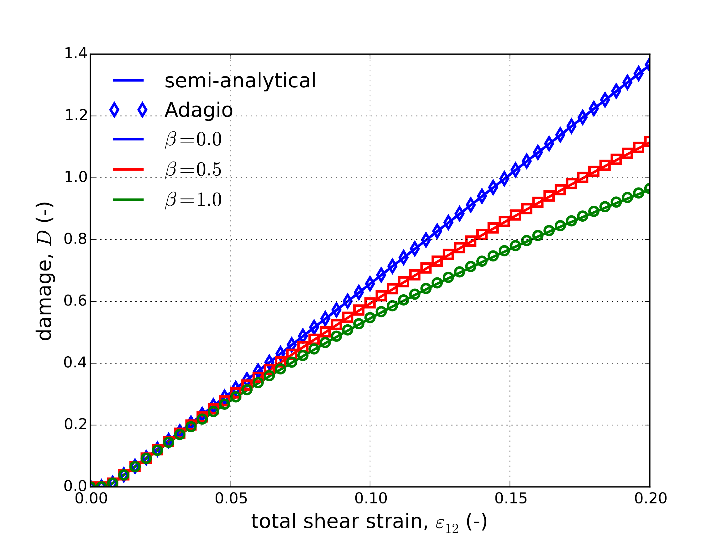
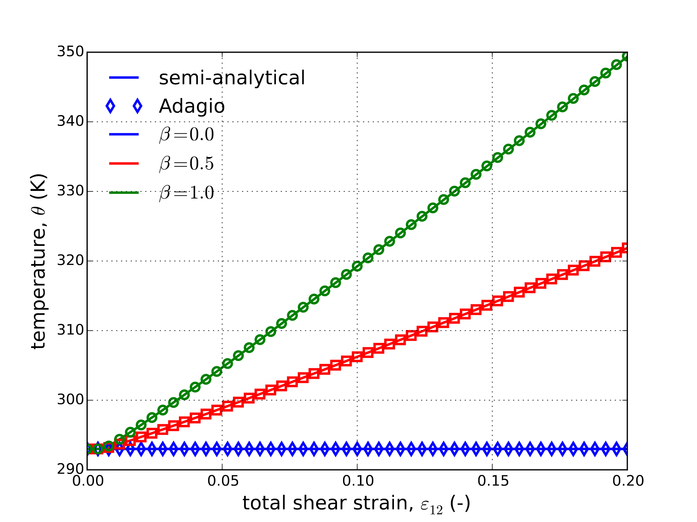
The effect of plastic work is considered for \(\omega=1\text{s}^{-1}\) in Fig. 4.36. Similar influences like those reported in the uniaxial stress case are observed. A larger increase in temperature through plastic loading is noted however. Regardless in both the results of Figures Fig. 4.35 and Fig. 4.36 clear agreement between numerical and semi-analytical is observed further verifying the current implementation of the Johnson-Cook model.

Stress-strain

Damage

Temperature

Fig. 4.36 Semi-analytical and numerical (a) stress-strain (b) damage and (c) temperature evolutions of the Johnson-Cook model subjected to a pure shear loading with three different plastic work conversion ratios, \(\beta\). The strain rate for all three cases is \(\dot{\varepsilon}=1\text{s}^{-1}\).

4.12.4. User Guide

BEGIN PARAMETERS FOR MODEL JOHNSON_COOK
  #
  # Elastic constants
  #
  YOUNGS MODULUS = <real>
  POISSONS RATIO = <real>
  SHEAR MODULUS  = <real>
  BULK MODULUS   = <real>
  LAMBDA         = <real>
  TWO MU         = <real>
  #
  # Yield surface parameters
  #
  YIELD STRESS       = <real>
  HARDENING CONSTANT = <real>
  HARDENING EXPONENT = <real>
  RATE CONSTANT      = <real>
  REFERENCE RATE     = <real> (0.001)
  EDOT_REF           = <real> (0.0)
  #
  # Failure strain parameters
  #
  D1 = <real> (0.0)
  D2 = <real> (0.0)
  D3 = <real> (0.0)
  D4 = <real> (0.0)
  D5 = <real> (0.0)
  #
  # Temperature softening commands
  #
  RHOCV                 = <real>
  BETA                  = <real>
  THERMAL EXPONENT      = <real>
  REFERENCE TEMPERATURE = <real>
  MELT TEMPERATURE      = <real>
  INITIAL TEMPERATURE   = <real>
  #
  FORMULATION = <int> (0)
  #
END [PARAMETERS FOR MODEL JOHNSON_COOK]

In the command blocks that define the Johnson-Cook model:

• The YIELD STRESS defines the stress for onset of yield and the plasticity.

• The HARDENING CONSTANT command line defines \(B\).

• The HARDENING EXPONENT command line defines \(N\)

• The RHOCV command line defines \({\rho}C_v\) which is the product of material density and specific heat.

• The material initial temperature is defined by the INITIAL TEMPERATURE command line. Note, the Johnson Cook material model temperature is NOT linked to the standard model “temperature” field that is set from BEGIN PRESCRIBED TEMPERATURE command blocks.

• The thermal exponent \(M\) is defined with the THERMAL EXPONENT command line. This exponent must be greater than zero.

• The reference temperature \(\theta_{ref}\) is defined with the REFERENCE TEMPERATURE command line.

• The melt temperature \(\theta_{melt}\) is defined with the MELT TEMPERATURE command line.

• The reference strain rate, \(\dot{\varepsilon}_{0}\), is defined with the REFERENCE RATE command line. The default is \(0.001 \, s^{-1}\).

• The fraction of plastic work that is converted to heat, \(\beta\), is defined with the BETA command line. The default is 0.95.

• The fracture coefficient \(D_{1}\) is defined with the D1 command line. The default is 0.0.

• The fracture coefficient \(D_{2}\) is defined with the D2 command line. The default is 0.0.

• The fracture coefficient \(D_{3}\) is defined with the D3 command line. The default is 0.0.

• The fracture coefficient \(D_{4}\) is defined with the D4 command line. The default is 0.0.

• The fracture coefficient \(D_{5}\) is defined with the D5 command line. The default is 0.0.

• The failure model – and corresponding coefficients – are only valid for solid (3D) elements. Specifying the values for 2D elements (e.g. shell) will result in an error as the damage model is not implemented. A possible alternative is the \(J_2\) Plasticity Model specified with Johnson-Cook hardening and failure.

• FORMULATION controls the strain rate source term. A FORMULATION of 0 is the default which is to use the total strain rate. A FORMULATION of 1 means use the plastic strain rate. The plastic strain rate is monotonic and changes a much lower frequency than the total strain rate, thus use of the plastic strain rate may be more stable.

4.12.4.1. Warnings and Usage Guidelines

Warning

Strongly rate dependent models may fare poorly in implicit quasistatic solution. In implicit the rate term used to evaluate the current load step is the rate seen by the model in the previous load step. Potentially this can cause the solution to jump back and forth between a high right and low rate equilibrium state from step to step.

Output variables available for this model are listed in Table 4.15.

Table 4.15 State Variables for JOHNSON COOK Model

Name	Description
RADIUS	radius of yield surface
EQPS	equivalent plastic strain
THETA	temperature
EQDOT	effective total strain rate
ITER
EFAIL	failure strain, \(\varepsilon^{f}\)
DAMAGE	damage, \(D\)
YIELD_STRESS	yield stress

---

[1]

G.R. Johnson and W.H. Cook. A constitutive model and data for metals subjected to large strains, high strain rates and high temperatures. In Proc. 7th. Int. Symp. on Ballistics, 541–547. The Hague, The Netherlands, 1983.

[2] (1,2)

G.R. Johnson and W.H. Cook. Fracture characteristics of three metals subjected to various strains, strain rates, temperatures and pressures. Engineering Fracture Mechanics, 21(1):31–48, 1985.

[3]

F.J. Zerilli and R.W. Armstrong. Dislocation-mechanics-based constitutive relations for material dynamics calculations. Journal of Applied Physics, 61:1816–1825, 1987.

[4]

D.J. Steinberg, S.G. Cochran, and M.W. Guinan. A constitutive model for metals applicable at high-strain rate. Journal of Applied Physics, 51:1498–1504, 1980.

[5]

D.J. Steinberg and C.M. Lund. A constitutive model for strain rates from 10$^-4$ to 10$^6$ s$^-1$. Journal of Applied Physics, 65:1528–1533, 1989.

[6]

A.A. Brown and D.J. Bammann. Validation of a model for static and dynamic recrystallization in metals. International Journal of Plasticity, 32–33:17–35, 2012.

[7]

P.S. Follansbee and U.F. Kocks. A constitutive description of the deformation of copper based on the use of the mechanical threshold stress and an internal state variable. Acta Metallurgica, 36(1):81–93, 1988.

[8]

P.S. Follansbee and G.T. Gray III. An analysis of the low temperature, low and high strain-rate deformation of Ti-6Al-4V. Metallurgical Transactions A, 20A:863–874, 1989.

[9] (1,2)

E. Corona and G. E. Orient. An evaluation of the Johnson-Cook model to simulate puncture of 7075 aluminum plates. Technical Report SAND2014-1550, Sandia National Laboratories, Albuquerque, NM, 2014. \href http://infoserve.sandia.gov/sand_doc/2014/141550.pdfpdf.