4.24. Soil and Foam Model

4.24.1. Theory

The soil and crushable foam model is a plasticity model that can be used for modeling soil, crushable foam, or other highly compressible materials. Given the right input, the model is a Drucker-Prager model.

For the soil and crushable foam model, the yield surface is a surface of revolution about the hydrostat in principal stress space. A planar end cap is assumed for the yield surface so that the yield surface is closed. The yield stress \(\sigma_{yd}\) is specified as a polynomial in pressure \(p\). The yield stress is given as:

(4.114)\[\sigma _{yd} = a_0 + a_1 p + a_2p^{2}\,,\]

where the pressure \(p\) is positive in compression. The determination of the yield stress from (4.114) places severe restrictions on the admissible values of \(a_{0}\), \(a_{1}\), and \(a_{2}\). There are three valid cases for the yield surface. In the first case, there is an elastic–perfectly plastic deviatoric response, and the yield surface is a cylinder oriented along the hydrostat in principal stress space. In this case, \(a_{0}\) is positive, and \(a_{1}\) and \(a_{2}\) are zero. In the second case, the yield surface is conical. A conical yield surface is obtained by setting \(a_{2}\) to zero and using appropriate values for \(a_{0}\) and \(a_{1}\). In the third case, the yield surface has a parabolic shape. For the parabolic yield surface, all three coefficients in (4.114) are nonzero. The coefficients are checked to determine that a valid negative tensile-failure pressure can be derived based on the specified coefficients.

For the case of the cylindrical yield surface (e.g., \(a_0 > 0\) and \(a_{1} = a_{2} = 0\)), there is no tensile-failure pressure. For the other two cases, the computed tensile-failure pressure may be too low. To handle the situations where there is no tensile-failure pressure or the tensile-failure pressure is too low, a pressure cutoff can be defined. If a pressure cutoff is defined, the tensile-failure pressure is the larger of the computed tensile-failure pressure and the defined cutoff pressure.

The plasticity theories for the volumetric and deviatoric parts of the material response are completely uncoupled. The volumetric response is computed first. The mean pressure \(p\) is assumed to be positive in compression, and a yield function \(\phi_{p}\) is written for the volumetric response as:

(4.115)\[\phi_p = p - f_p \left( {\varepsilon _{V} } \right)\,,\]

where \(f_p \left( {\varepsilon _{V} } \right)\) defines the volumetric stress-strain curve for the pressure. The yield function \(\phi_{p}\) determines the motion of the end cap along the hydrostat.

4.24.2. Implementation

The soil and crushable foam model is a rate-independent, hypoelastic model that splits and sequentially evaluates the volumetric and deviatoric response. To determine the inelastic flow, an elastic predictor-inelastic corrector approach is adopted for each of the aforementioned responses.

For the volumetric response, an updated logarithmic volume strain, \(\varepsilon^{n+1}_{v}\), is computed by,

\[\varepsilon^{n+1}_{v}=\varepsilon^{n}_{v}-\Delta td_{kk}.\]

Note, in this case, the volume strain is defined such that it is positive in compression. This strain value is then used to evaluate the volumetric yield function defined in (4.115) and determine the appropriate pressure, \(p\), the material is subject to.

To evaluate the deviatoric response, a trial deviatoric stress, \(s^{tr}_{ij}\), is defined as,

\[s^{tr}_{ij}=s^n_{ij}+2\mu\hat{d}_{ij}\Delta t,\]

with \(\hat{d}_{ij}\) being the deviatoric part of the unrotated rate of deformation. The deviatoric yield function, \(f\), is then used to evaluate if any deviatoric plastic flow is occurring and is written as,

\[f\left(s_{ij},p\right)=\phi\left(s_{ij}\right)-\sigma_{yd}\left(p\right),\]

where \(\sigma_{yd}\) is the yield stress given in (4.114) and \(\phi\left(s_{ij}\right)\) the effective stress given as,

\[\phi\left(s_{ij}\right)=\sqrt{\frac{3}{2}s_{ij}s_{ij}}.\]

If an elastic response is evident (\(f\leq 0\)), then the final stress is simply,

\[T^{n+1}_{ij}=s^{tr}_{ij} - p\delta_{ij}.\]

Otherwise, if a plastic response is observed, a radial return approach like that discussed in Section 4.7.2 is utilized to find the equivalent plastic strain increment, \(\Delta\bar{\varepsilon}^p\). Unlike that case, given the decoupling between the volumetric and deviatoric behaviors, the hardening component of the yield surface does not change leading to an expression of the form,

\[\Delta\bar{\varepsilon}^p=\frac{f}{3\mu},\]

and the final stress is,

\[T^{n+1}_{ij}=s^{tr}_{ij}-3\mu\Delta\bar{\varepsilon}^p\frac{s^{tr}_{ij}}{\phi}-p\delta_{ij}.\]

4.24.3. Verification

The soil and foam model is verified for a triaxial compression load path. First the material is biaxially loaded in plane strain using load control, then the prescribed loads are released while the material is compressed in displacement control.

4.24.3.1. Triaxial Compression

The soil and foam model is tested in triaxial compression. For this problem, both lateral stresses, \(\sigma_{11}\) and \(\sigma_{33}\), are prescribed along with the axial strain, \(\varepsilon_{22}\). Furthermore, the lateral stresses are equal, \(\sigma_{11} = \sigma_{33}\). For the elastic response, the axial stress is

\[\sigma_{22} = E \varepsilon_{22} + 2\nu \sigma_{11}\]

where \(E\) is the elastic modulus and \(\nu\) is the Poisson’s ratio. The lateral strains are

\[\varepsilon_{11} = -\nu \left( \varepsilon_{22} - \sigma_{11}/\lambda \right)\]

where \(\lambda\) is the Lame constant.

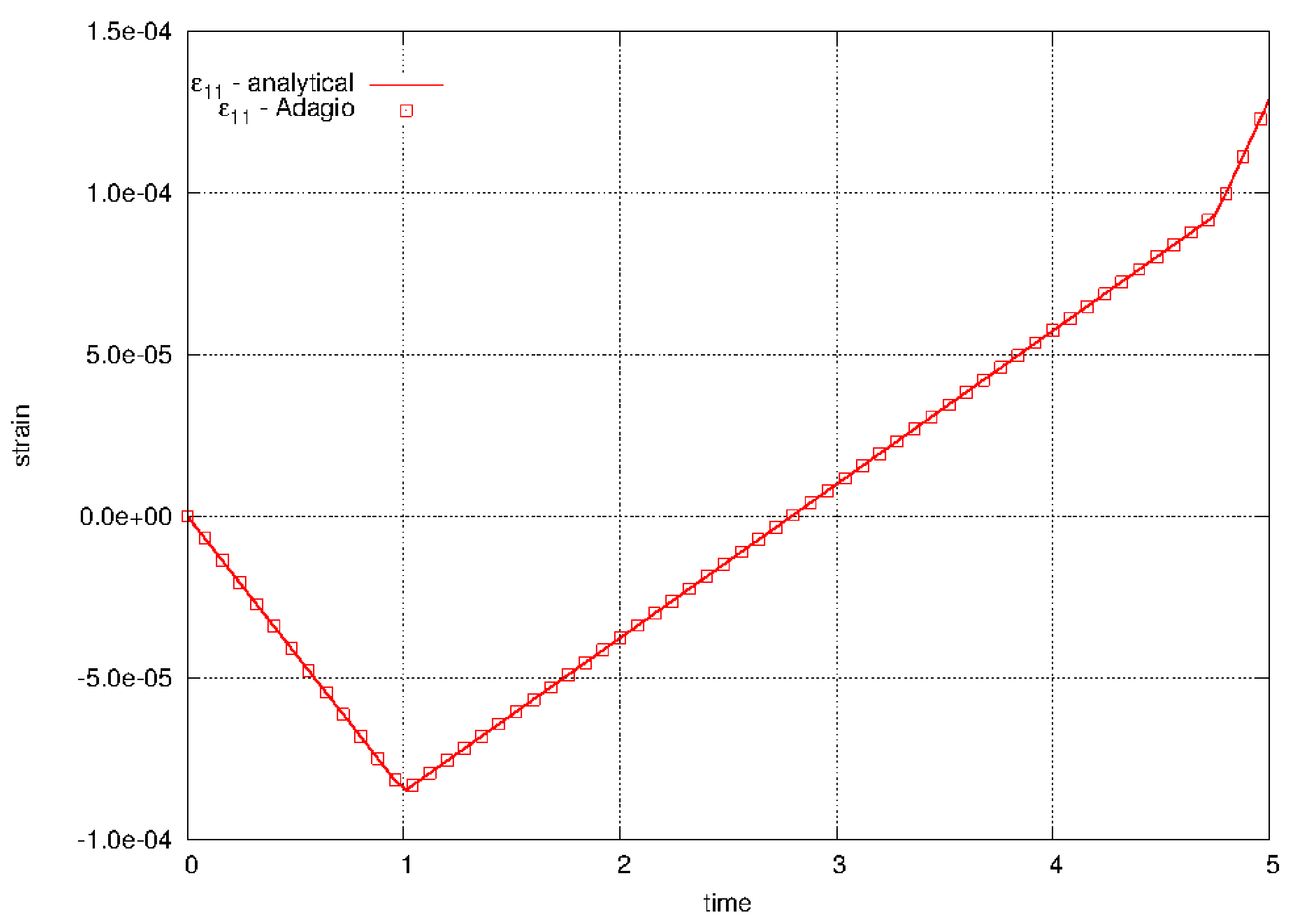
../../_images/soil_and_foam_triaxial1.png — Fig. 4.115 Lateral strain, \(\varepsilon_{11}\) and \(\varepsilon_{33}\), over the course of the prescribed triaxial loading path.

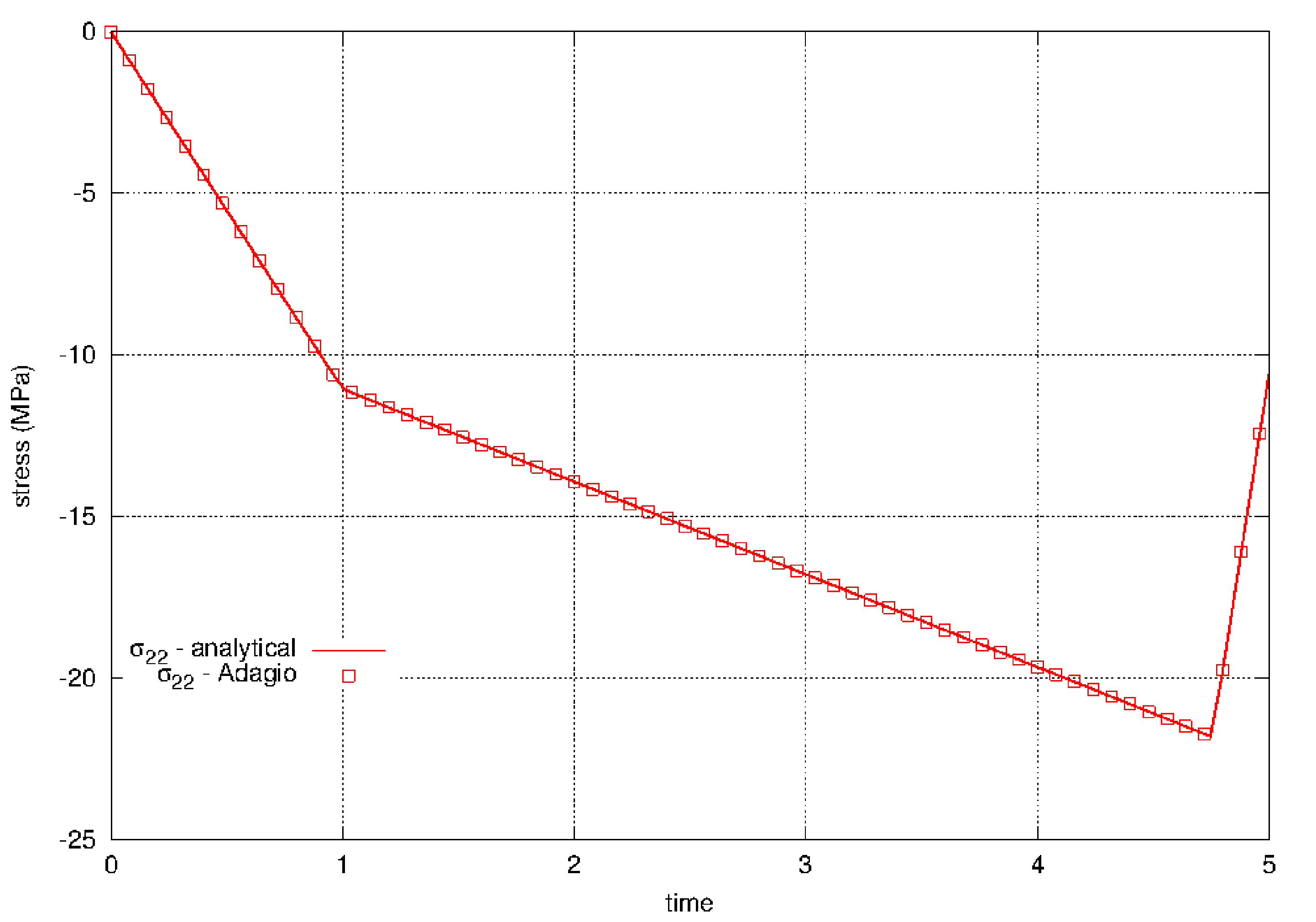
../../_images/soil_and_foam_triaxial2.png — Fig. 4.116 Axial stress, \(\sigma_{22}\), over the course of the prescribed triaxial loading path.

4.24.4. User Guide

BEGIN PARAMETERS FOR MODEL SOIL_FOAM
  #
  # Elastic constants
  #
  YOUNGS MODULUS = <real>
  POISSONS RATIO = <real>
  SHEAR MODULUS  = <real>
  BULK MODULUS   = <real>
  LAMBDA         = <real>
  TWO MU         = <real>
  #
  # Yield surface parameters
  #
  A0 = <real>
  A1 = <real>
  A2 = <real>
  PRESSURE CUTOFF   = <real>
  PRESSURE FUNCTION = <string>
END [PARAMETERS FOR MODEL SOIL_FOAM]

In the above command blocks:

The constant coefficient in the equation for the yield surface ( (4.114)) is defined with the A0 command line.
The coefficient for the linear term in the equation for the yield surface ( (4.114)) is defined with the A1 command line.
The coefficient for the quadratic term in the equation for the yield surface ( (4.114)) is defined with the A2 command line.
The user-defined maximum tensile-failure pressure is defined with the PRESSURE CUTOFF command line.
The pressure as a function of volumetric strain is defined with the function named on the PRESSURE FUNCTION command line.

For information about the soil and crushable foam model, see the PRONTO3D document listed as Reference [[1]]. The soil and crushable foam model is the same as the soil and crushable foam model in PRONTO3D. The PRONTO3D model is based on a material model developed by Krieg [[2]]. The Krieg version of the soil and crushable foam model was later modified by Swenson and Taylor [[3]]. The soil and crushable foam model developed by Swenson and Taylor is the model in PRONTO3D and is also the shared model for Presto and Adagio.

Output variables available for this model are listed in Table 4.36.

Table 4.36 State Variables for SOIL FOAM Model
Name	Description
`EVOL_MAX`	maximum volumetric strain seen by the material point
`EVOL_FRAC`	volumetric strain for tensile fracture
`EVOL`	current volumetric strain
`EQPS`	equivalent plastic strain