4.20. Viscoplastic Model

4.20.1. Theory

The viscoplastic model is a rate dependent plasticity model that is useful for modeling solders and brazes and was developed by Neilsen et al. [[1]]. This model is formulated in terms of the stress rate for the material. Like many inelastic models, the rate of deformation, \(D_{ij}\), is additively decomposed into an elastic, \(D_{ij}^{\text{e}}\), and an inelastic, \(D_{ij}^{\text{in}}\) part such that,

\[D_{ij} = D_{ij}^{\text{e}} + D_{ij}^{\text{in}}.\]

The elastic rate of deformation is the only part that contributes to the stress rate and it does so through the elastic moduli, \(\mathbb{C}_{ijkl}\), in a linear fashion leading to the relation,

(4.80)\[\stackrel{\circ}{\sigma}_{ij} = \mathbb{C}_{ijkl} D_{kl}^{\text{e}},\]

where \(\mathbb{C}_{ijkl}\) are the components of the fourth-order, isotropic elasticity tensor. The stress rate is arbitrary, as long as it is objective. Two objective stress rates are commonly used: the Jaumann rate and the Green-McInnis rate. For problems with fixed principal axes of deformation, these two rates give the same answers. For problems where the principal axes of deformation rotate during the deformation, the two rates can give different answers. Generally speaking there is no reason to pick one objective rate over another.

The inelastic strain rate is a function of the stress state, \(\sigma_{ij}\), the temperature, \(\theta\), and a number of internal state variables including both scalar isotropic, \(D\), and tensorial kinematic, \(B_{ij}\), hardening variables. With these dependencies defined, a general form for the evolution of the inelastic deformation may be given by,

\[D_{ij}^{\text{in}} = \frac{3}{2} \gamma\left( \sigma_{ij}, \theta; D, B_{ij} \right) n_{ij},\]

where \(n_{ij}\) is the direction of inelastic deformation and is defined as,

(4.81)\[n_{ij}=\frac{1}{\tau}\left(s_{ij}-\frac{2}{3}B_{ij}\right),\]

and

\[\tau=\sqrt{\frac{3}{2}\left(s_{ij}-\frac{2}{3}B_{ij}\right)\left(s_{ij}-\frac{2}{3}B_{ij}\right)},\]

with \(s_{ij}\) being the deviatoric stress tensor. The inelastic strain rate, \(\gamma\), is defined via a hyperbolic sin law,

(4.82)\[\gamma = f(\theta)\left[ \sinh\left( \frac{\tau}{\alpha(\theta) D} \right) \right]^{p(\theta)},\]

where \(f(\theta) = \exp(g(\theta))\). The expressions \(g(\theta)\), \(\alpha(\theta)\), and \(p(\theta)\) are model parameters that are functions of temperature.

The evolution laws for the state variables \(D\) and \(B_{ij}\) are,

(4.83)\[\dot{D} = \frac{A_{1}}{\left( D-D_{0} \right)^{A_{3}}}\gamma - A_{2}\left( D-D_{0} \right)^{2},\]

and

(4.84)\[\dot{B}_{ij} = \frac{A_{4}}{b^{A_{6}}} D_{ij}^{\text{in}} - A_{5} b B_{ij},\]

where

\[b = \sqrt{\frac{2}{3}B_{ij}B_{ij}}.\]

The parameters \(D_{0}\), \(A_{1}\), \(A_{2}\), \(A_{3}\), \(A_{4}\), \(A_{5}\) and \(A_{6}\) are model parameters. The parameters \(A_{1}\), \(A_{2}\), \(A_{4}\) and \(A_{5}\) are also functions of temperature. The model can be simplified with the appropriate choice of these parameters.

The following material parameters are functions of temperature and have the following form

\[\begin{split}G(\theta) = G_{0} h_{G}(\theta) \;\;\; ; \;\;\; K(\theta) = K_{0} h_{K}(\theta) \nonumber \\ \nonumber \\ g(\theta) = g_{0} h_{g}(\theta) \;\;\; ; \;\;\; p(\theta) = p_{0} h_{p}(\theta) \;\;\; ; \;\;\; \alpha (\theta) = \alpha_{0} h_{\alpha}(\theta) \nonumber \\ \\ A_{1} (\theta) = A_{1}^{0} h_{1}(\theta) \;\;\; ; \;\;\; A_{2} (\theta) = A_{2}^{0} h_{2}(\theta) \nonumber \\ \nonumber \\ A_{4} (\theta) = A_{4}^{0} h_{4}(\theta) \;\;\; ; \;\;\; A_{5} (\theta) = A_{5}^{0} h_{5}(\theta) \nonumber\end{split}\]

where the functions \(h_{*}(\theta)\) are normalized functions of temperature and the values \((*)_{0}\) or \((*)^{0}\) are the reference values that are input in the command block.

4.20.2. Implementation

An explicit, forward Euler scheme is used to integrate the viscoplastic model. First, during initialization, the isotropic hardening variable \(D\) is set to \(1.001 D_{0}\). This is done to avoid a singularity in (4.83). Additionally, the kinematic variable is set to zero (\(B_{ij}=0\)).

Like the power law creep model that is integrated in a similar fashion, the chosen numerical scheme is conditionally stable. As detailed in [[1]], a critical stability time step of,

\[\Delta t_{n+1}\leq\frac{2\alpha\left(\theta\right)D}{3Gf\left(\theta\right)p\left(\theta\right)\sinh^{p\left(\theta\right)-1}\left(\frac{\tau}{\alpha\left(\theta\right)D}\right)\cosh\left(\frac{\tau}{\alpha\left(\theta\right)D}\right)},\]

may be determined. For convince, in the following the dependence of \(f,~p,\) and \(\alpha\) will be assumed and not explicitly written. Instead, \(f^{n+1}\) will be used to refer to \(f\left(\theta^{n+1}\right)\). Two additional limits are also imposed to ensure accurate integration of the state variables. Specifically,

\[\Delta t_{n+1}\leq\sqrt{\frac{2\delta D_0\Delta t_n}{|\dot{D}_n-\dot{D}_{n-1}|}},\]

and

\[\Delta t_{n+1}\leq\sqrt{\frac{2\delta D_0\Delta t_n}{|\dot{b}_n-\dot{b}_{n-1}|}},\]

where \(\delta\) is an allowable error measure (here, \(1.0x10^{-3}\)) and \(\dot{x}_n\) refers to the time rate of change of variable \(x\) at time step \(n\). The current time step is checked to ensure it meets those criteria or else it is scaled back to ensure accurate integration.

After assessing the acceptability of the time step, the new material state at time \(t=t_{n+1}\) is determined. If the time step needs to be cut back, multiple sub-increments are used. To elaborate, let \(k\) denote a specific sub-increment and \(N\) represent the total number of sub-increments. Each \(k^{th}\) interval evaluates the numerical routine over a step size \(\delta t^k\) where \(\Delta t =\sum_{k=0}^N\delta t^k\). In such cases, temperature dependent variables are linearly interpolated between their values at \(t_n\) and \(t_{n+1}\). For example,

\[G^k=G_n+\frac{\Delta t^k}{\Delta t}\left(G_{n+1}-G_n\right),\]

where \(\Delta t^k\) is the current sub-increment time, \(\Delta t^k=\sum_{r=0}^k\delta t^r\). For simplicity and clarity of presentation, in the discussion below it is assumed that the input time step is acceptable and only a single increment is needed. If additional sub-increments were needed, the below steps would be repeated \(N\) times with time intervals of \(\delta t^k\).

It is first noted that the unrotated stress, \(T_{ij}\), and deformation rate, \(d_{ij}\), may be decomposed as,

\[\begin{split}T^n_{ij}=-p^n\delta_{ij}+s^n_{ij}, \\ d^n_{ij}=\frac{1}{3}d^n_{kk}\delta_{ij}+\hat{d}^n_{ij},\end{split}\]

with \(p\) being the pressure (\(p=-\frac{1}{3}T_{kk}\)) and \(\hat{d}_{ij}\) being the rate of deviatoric deformation. As the inelastic deformation flows in a deviatoric direction, the hydrostatic and deviatoric components may be evaluated separately. With this in mind, the pressure may be easily integrated via,

\[p^{n+1}=p^n\frac{K^{n+1}}{K^n}+\frac{1}{2}\left(K^n+K^{n+1}\right)d_{kk}\Delta t,\]

where \(K^n\) is abbreviated notation for \(K\left(\theta^{n}\right)\). The inelastic deformation rate is then determined as,

\[D^{\text{in}}_{ij}=\frac{3}{2}\gamma\left(\sigma_{ij}^n,\theta^n;D^n,B^n_{ij}\right)n^{n}_{ij},\]

by evaluating expressions (4.81)-(4.82) at \(t=t_n\) and \(\theta=\theta^n\). The internal state variables may then be similar evolved via (4.83) and (4.84). With the inelastic state determined, the updated deviatoric stress may be found via,

\[s_{ij}^{n+1}=\frac{G^{n+1}}{G^n}s_{ij}^n+2\Delta t G^{n}\left(\hat{d}_{ij}-D^{\text{in}}_{ij}\right),\]

with the updated stress being,

\[T^{n+1}_{ij}=-p^{n+1}\delta_{ij}+s^{n+1}_{ij}.\]

4.20.3. Verification

The viscoplastic model is verified through two, time-dependent tests – creep and stress relaxation. To simplify the problem for verification purposes, the isothermal response only considering isotropic hardening and recovery is investigated. It is noted, however, that given the stress dependence and evolving internal state variable in the inelastic strain rate, a closed-form analytical solution may not be found. Semi-analytical approaches numerically integrating the differential equations are easily obtainable and used for comparison purposes. The considered test temperature is 450\(^{\circ}`C (:math:`723\) K) and material properties and model parameters are those of CusilABA taken from Table 3 of [[1]] and are reproduced for convenience below in Table 4.30.

Table 4.30 Material properties and model parameters used for isothermal, isotropic hardening/recovery creep and stress

\(E\)	77.8 GPa	\(\nu\)	0.375
\(g\)	-13.88	\(p\)	2.589
\(A_1\)	\(3x10^4\) MPa\(^{A_3+1}\)	\(A_2\)	\(2.07x10^{-5}\) \(\frac{1}{\text{MPa s}}\)
\(A_3\)	1.746	\(D_0\)	50.0 MPa
\(A_4\)	0 MPa\(^{A_6+1}\)	\(A_5\)	0.0 \(\frac{1}{\text{MPa s}}\)
\(A_6\)	0.0	\(\alpha\)	\(1.0\)

4.20.3.1. Creep

The creep response of the viscoplastic model is investigated both numerically and semi-analytically. For such a loading, the stress tensor is \(\sigma_{ij}=\sigma\left(t\right)\delta_{i1}\delta_{j1}\) with \(\sigma\left(t\right)\) being a prescribed quantity. For this study, \(\sigma\left(t\right)\) ramps linearly from \(0\) to \(\sigma_{max}\) over the interval \(t=[0,100~\text{s}]\) with \(\sigma_{max}=300\) MPa. That magnitude is then maintained for the next 900 s.

To analytically determine the model response, the constitutive law (4.80) is inverted to yield

(4.85)\[D_{ij}=\mathbb{S}_{ijkl}\dot{\sigma}_{kl}+D^{\text{in}}_{ij},\]

and it is trivial to determine that

(4.86)\[\mathbb{S}_{ijkl}\dot{\sigma}_{kl}=\dot{\sigma}\mathbb{S}_{11kl}.\]

For the inelastic response, for the purely isotropic case it is noted that \(\tau=\sigma\left(t\right)\) and therefore \(n_{ij}=\frac{2}{3}\left[\delta_{i1}\delta_{j1}-\frac{1}{2}\left(\delta_{i2}\delta_{j2}+\delta_{i3}\delta_{j3}\right)\right]\). Additionally, the inelastic strain rate reduces to,

(4.87)\[\gamma=f\left[\sinh\left(\frac{\sigma\left(t\right)}{\alpha D}\right)\right]^p\]

producing a rate of inelastic deformation of,

(4.88)\[D^{\text{in}}_{ij}=\gamma\left[\delta_{i1}\delta_{j1}-\frac{1}{2}\left(\delta_{i2}\delta_{j2}+\delta_{i3}\delta_{j3}\right)\right].\]

Expressions (4.85), (4.86), (4.88), and (4.83) can be easily integrated (via forward Euler or Runge-Kutta) to determine a semi-analytical response. Both the numerical and semi-analytical responses of the strain and stress (including flow stress, \(D\)) are presented below in Fig. 4.97(a) and Fig. 4.97(b), respectively.

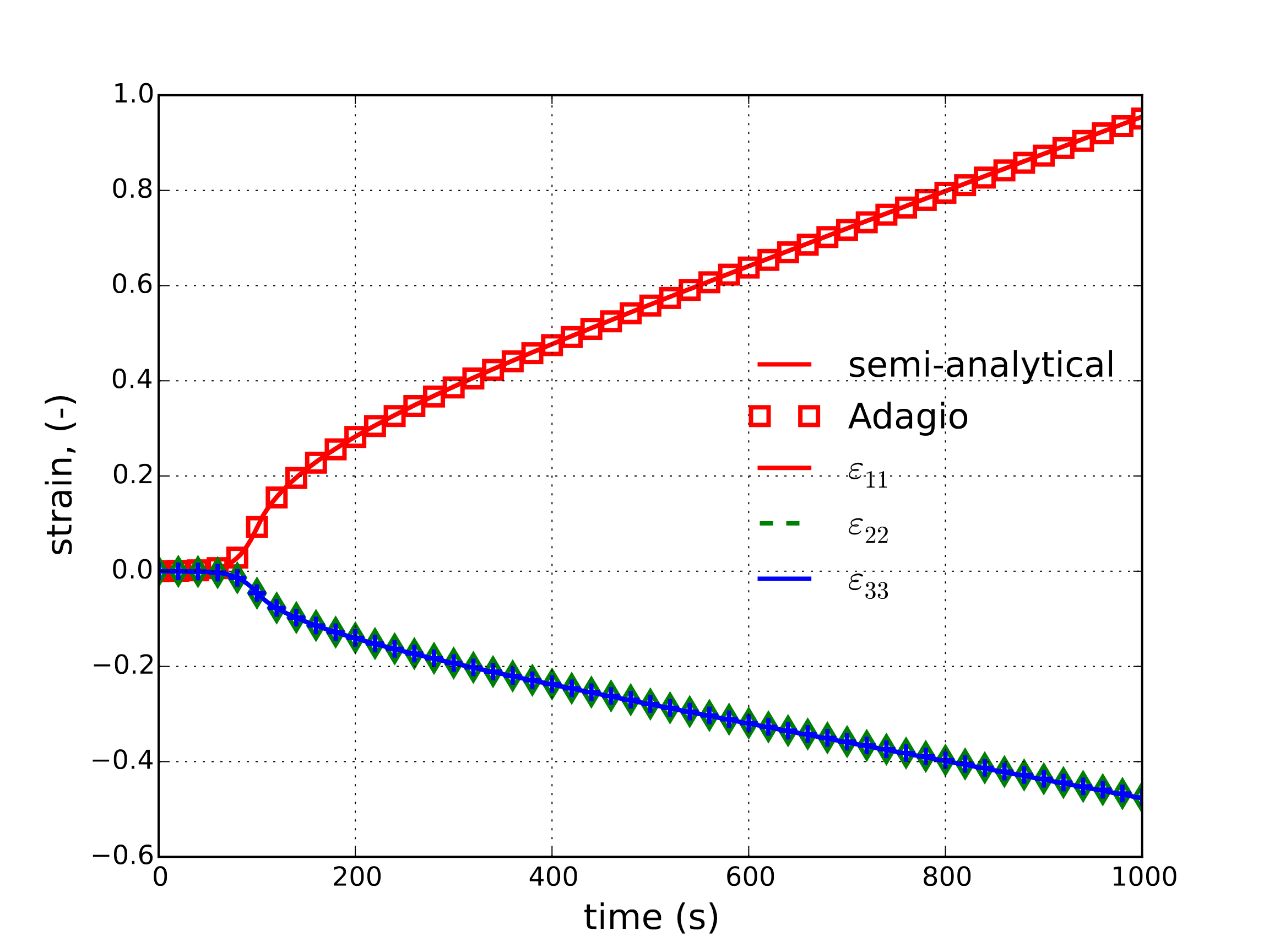Strain

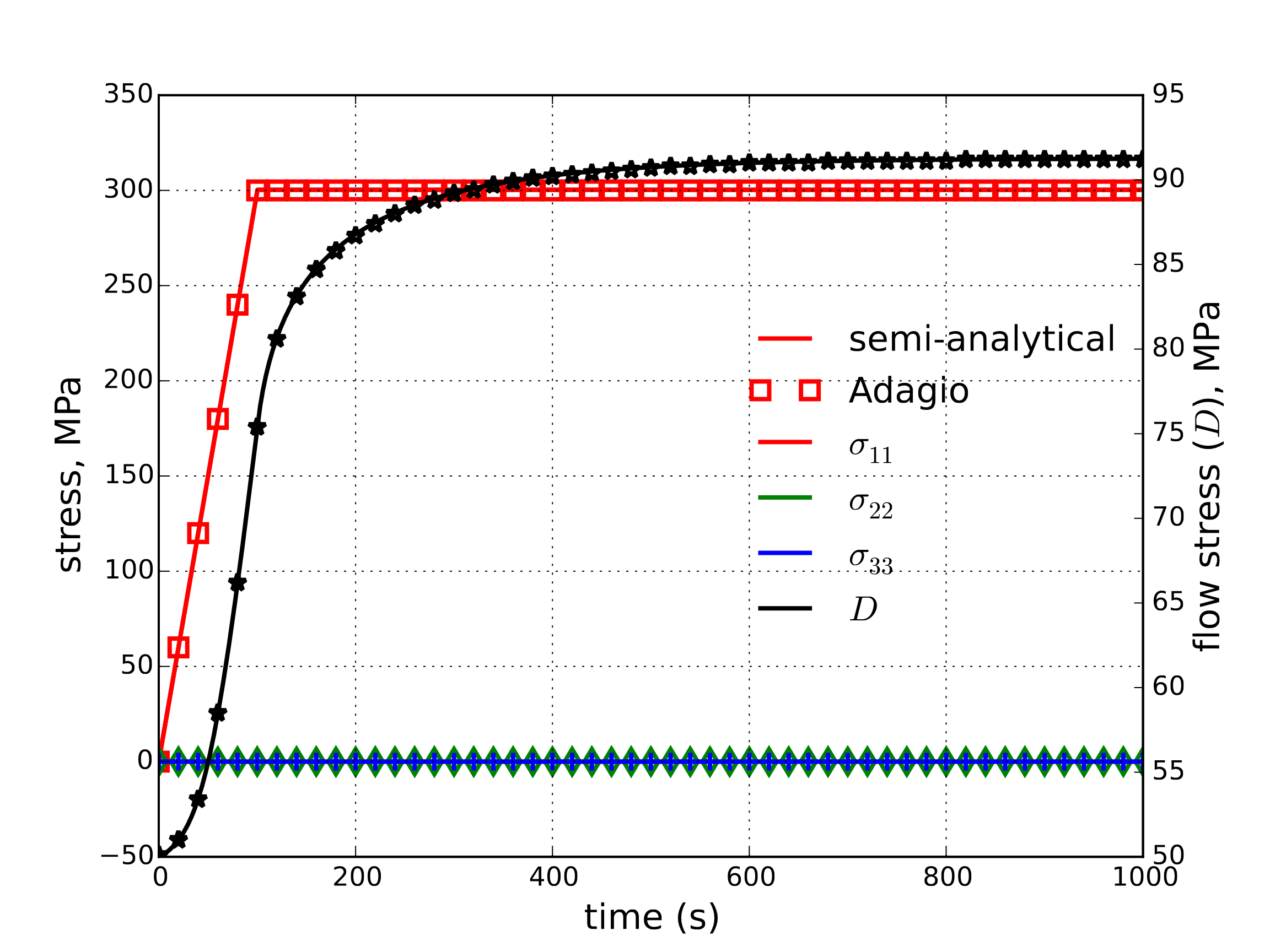Stress

Fig. 4.97 Semi-analytical and numerical results of (a) strain and (b) external and internal, (\(D\)), stress evolution during a creep test with the viscoplastic model.

4.20.3.2. Stress Relaxation

The model response through a stress relaxation type loading is considered here both numerically and semi-analytically. For this purpose, a displacement controlled loading, \(u_1=\lambda\left(t\right)\), is employed. The other displacement degrees of freedom are not prescribed to ensure that a uniaxial stress state (\(\sigma_{ij}=\sigma\left(t\right)\delta_{i1}\delta_{j1}\)) develops. Specifically, the displacement is set to scale linearly over 100 s (from \(t=0\) to \(t=100\) s) obtaining a maximum of \(u_1=0.01\) at \(t=100\) s. Initially, a unit length is assumed. This displacement is held fixed over the next 900 s to investigate the stress relaxation characteristics of the model.

A similar procedure to the power law creep model (Section 4.19.3.2) is employed here. Specifically, by noting the elastic isotropy, uniaxial stress state, and (4.88) the elastic deformation rate in the direction of loading (\(D^{\text{e}}_{11}\)) is found to be,

\[D^{\text{e}}_{11}=\frac{\dot{\lambda}\left(t\right)}{1+\lambda\left(t\right)}-\gamma,\]

where an expression for \(\gamma\) is given in (4.87). By noting \(\dot{\sigma}_{ij}=\mathbb{C}_{ijkl}D^{\text{e}}_{kl}\) and \(D_{ij}=D^{\text{e}}_{ij}+D^{\text{in}}_{ij}\), the material state may easily be found via numerical integration. The result strain and stress evolutions are given in Fig. 4.98(a) and Fig. 4.98(b), respectively.

Strain

Stress

Fig. 4.98 Semi-analytical and numerical results of (a) strain and (b) external and internal (\(D\)) stress evolution during a stress relaxation test with the viscoplastic model.

4.20.4. User Guide

BEGIN PARAMETERS FOR MODEL VISCOPLASTIC
  #
  # Elastic constants
  #
  YOUNGS MODULUS = <real>
  POISSONS RATIO = <real>
  SHEAR MODULUS  = <real>
  BULK MODULUS   = <real>
  LAMBDA         = <real>
  TWO MU         = <real>

  FLOW RATE     = <real>
  SINH EXPONENT = <real>
  ALPHA         = <real>
  ISO HARDENING = <real>
  ISO RECOVERY  = <real>
  ISO EXPONENT  = <real>
  KIN HARDENING = <real>
  KIN RECOVERY  = <real>
  KIN EXPONENT  = <real>
  FLOW STRESS   = <real>

  SHEAR FUNCTION    = <string>
  BULK FUNCTION     = <string>
  RATE FUNCTION     = <string>
  EXPONENT FUNCTION = <string>
  ALPHA FUNCTION    = <string>
  IHARD FUNCTION    = <string>
  IREC FUNCTION     = <string>
  KHARD FUNCTION    = <string>
  KREC FUNCTION     = <string>
  MAX SUBINCREMENTS = <int> itmax (2000)
END [PARAMETERS FOR MODEL VISCOPLASTIC]

In the above command blocks:

• Since the model requires functions to describe the temperature dependence of the bulk and shear modulus, it is recommended that one inputs the bulk and shear modulus at some reference temperature. However, any two of the elastic constants can be used for input.

• The reference value in the equation for the flow rate, \(\ln f_{0}\), is defined with the FLOW RATE command line.

• The reference value for the exponent on the \(\sinh\) function, \(p_{0}\), is defined with the SINH EXPONENT command line.

• The reference value \(alpha_{0}\) is defined with the ALPHA command line.

• The reference value for the isotropic hardening parameter, \(A_{1}^{0}\), is defined with the ISO HARDENING command line.

• The reference value for the isotropic recovery parameter, \(A_{2}^{0}\), is defined with the ISO RECOVERY command line.

• The value for the isotropic hardening exponent parameter, \(A_{3}\), is defined with the ISO EXPONENT command line.

• The reference value for the kinematic hardening parameter, \(A_{4}^{0}\), is defined with the KIN HARDENING command line.

• The reference value for the kinematic recovery parameter, \(A_{5}^{0}\), is defined with the KIN RECOVERY command line.

• The value for the kinematic hardening exponent parameter, \(A_{6}\), is defined with the KIN EXPONENT command line.

• The value for the flow stress, \(D_{0}\), is defined with the FLOW STRESS command line.

• The user-defined and normalized function that gives the shear modulus as a function of temperature, \(h_{G}(\theta)\), is defined with the SHEAR FUNCTION command line.

• The user-defined and normalized function that gives the bulk modulus as a function of temperature, \(h_{K}(\theta)\), is defined with the BULK FUNCTION command line.

• The user-defined and normalized function that gives the flow rate as a function of temperature, \(h_{g}(\theta)\), is defined with the RATE FUNCTION command line.

• The user-defined and normalized function that gives the \(\sinh\) exponent as a function of temperature, \(h_{p}(\theta)\), is defined with the EXPONENT FUNCTION command line.

• The user-defined and normalized function that gives \(\alpha\) as a function of temperature, \(h_{\alpha}(\theta)\), is defined with the ALPHA FUNCTION command line.

• The user-defined and normalized function that gives \(A_{1}\) as a function of temperature, \(h_{1}(\theta)\), is defined with the IHARD FUNCTION command line.

• The user-defined and normalized function that gives \(A_{2}\) as a function of temperature, \(h_{2}(\theta)\), is defined with the IREC FUNCTION command line.

• The user-defined and normalized function that gives \(A_{4}\) as a function of temperature, \(h_{4}(\theta)\), is defined with the KHARD FUNCTION command line.

• The user-defined and normalized function that gives \(A_{5}\) as a function of temperature, \(h_{5}(\theta)\), is defined with the KREC FUNCTION command line.

• The Viscoplastic model may need to take sub-increments to solve for the plastic flow over the current time step. The maximum number of steps that may be taken on a step prior to issuing an error can be set by the MAX SUBINCREMENTS command line. This value defaults to 2000.

Output variables available for this model are listed in Table 4.31.

More information on the model can be found in the report by Neilsen, et. al. [[1]].

Table 4.31 State Variables for VISCOPLASTIC Model

Name	Description
EQPS	equivalent plastic strain
SVB	kinematic hardening variable, \({\bf B}\)
SVB_XX	kinematic hardening variable - xx component, \(B_{xx}\)
SVB_YY	kinematic hardening variable - yy component, \(B_{yy}\)
SVB_ZZ	kinematic hardening variable - zz component, \(B_{zz}\)
SVB_XY	kinematic hardening variable - xy component, \(B_{xy}\)
SVB_YZ	kinematic hardening variable - yz component, \(B_{yz}\)
SVB_ZX	kinematic hardening variable - zx component, \(B_{zx}\)
SVD	isotropic hardening variable, \(D\)
EQDOT	inelastic strain rate, \(\gamma\)
COUNT	number of sub-increments
SHEAR	shear modulus, \(G(\theta)\)
BULK	bulk modulus, \(K(\theta)\)
RATE	\(g(\theta)\) (see (4.82))
EXP	\(p(\theta)\) (see (4.82))
ALPHA	\(\alpha(\theta)\) (see (4.82))
A1	isotropic hardening parameter, \(A_{1}(\theta)\)
A2	isotropic recovery parameter, \(A_{2}(\theta)\)
A4	kinematic hardening parameter, \(A_{4}(\theta)\)
A5	kinematic recovery parameter, \(A_{5}(\theta)\)

---

[1] (1,2,3,4)

M.K. Neilsen, S. N. Burchett, C. M. Stone, and J. J. Stephens. A viscoplastic theory for braze alloys. Technical Report SAND96-0984, Sandia National Laboratories, Albuquerque, NM, 1996. \href http://infoserve.sandia.gov/sand_doc/1996/960984.pdfpdf.