4.30. Orthotropic Crush Model

4.30.1. Theory

The orthotropic crush model in LAMÉ is designed to model the energy absorbing capability of crushable orthotropic materials, e.g. aluminum honeycomb, and is empirically based. The formulation follows that used for metallic honeycomb materials in LS-DYNA [[1]]. Three response regimes are assumed for this material: (i) orthotropic elastic, (ii) crush, and (iii) complete compaction (fully crushed). During the elastic regime, the model exhibits the response of an elastic, orthotropic material with all Poisson’s ratio equal to zero. After full compaction, the response is taken to be that of an isotropic, perfectly plastic material and the response between these two stages is tailored to smoothly transition between the two extremes. Crushing, incorporating both nonlinear elastic and plastic-like behaviors, is taken to begin as soon as volumetric contraction is noted (\(J=\det\left(F_{ij}\right)<1\)). As such, the purely elastic response is primarily seen during cyclic loadings in which the material is unloaded. An internal state variable, \(J_c\), is introduced to track the crushed state of the material and is defined as the minimum \(J\) over the entire deformation history such that,

\[J_c=\min_{t>0}\left[J\left(t\right)\right].\]

The crushing process manifests through two distinct behaviors: (i) the elastic properties scale linearly with the crush state from the initial orthotropic state to the of the final isotropic completely compacted material; and (ii) a plastic-like response is observed associated with corresponding crush curves (analogous to hardening curves).

Before complete compaction, the incremental constitutive relation may be written in terms of the rate of deformation tensor, \(D_{ij}\), as,

(4.142)\[\begin{split}\left\{ \begin{matrix} \stackrel{\circ}{\sigma}_{11} \\ \stackrel{\circ}{\sigma}_{22} \\ \stackrel{\circ}{\sigma}_{33} \\ \stackrel{\circ}{\sigma}_{12} \\ \stackrel{\circ}{\sigma}_{23} \\ \stackrel{\circ}{\sigma}_{31} \end{matrix} \right\} = \left[ \begin{matrix} \hat{E}_{11} & 0 & 0 & 0 & 0 & 0 \\ 0 & \hat{E}_{22} & 0 & 0 & 0 & 0 \\ 0 & 0 & \hat{E}_{33} & 0 & 0 & 0 \\ 0 & 0 & 0 & 2\hat{G}_{12} & 0 & 0 \\ 0 & 0 & 0 & 0 & 2\hat{G}_{23} & 0 \\ 0 & 0 & 0 & 0 & 0 & 2\hat{G}_{31} \end{matrix} \right] \left\{ \begin{matrix} D_{11} \\ D_{22} \\ D_{33} \\ D_{12} \\ D_{23} \\ D_{31} \end{matrix} \right\}\end{split}\]

where \(\hat{E}_{11}\), \(\hat{E}_{22}\), and \(\hat{E}_{33}\) are the normal stiffness and \(\hat{G}_{12}\), \(\hat{G}_{23}\), and \(\hat{G}_{31}\) are the shear stiffness. A clear decoupling between the different directional components is evident in (4.142). All six stiffness components are assumed to be functions of the current compaction level which may be defined as \(1-J_c\) and the evolution of these terms is responsible for crushing behavior \((*i*)\) alluded to previously.

The functional forms of the stiffness are given by,

(4.143)\[\begin{split}\hat{E}_{\beta} & = E_{\beta}+\alpha\left(E-E_{\beta}\right)\qquad\qquad \beta=11,~22,~33 \nonumber \\ \hat{G}_{\gamma} & = G_{\gamma}+\alpha\left(G-G_{\gamma}\right)\qquad\qquad \gamma=12,~23,~31,\end{split}\]

where \(E\) and \(G\) are the Young’s and shear moduli, respectively, of the fully compacted material while \(E_{\beta}\) and \(G_{\gamma}\) are the input orthotropic elastic stiffness components of the virgin, uncompacted material. It is assumed that these stiffness vary linearly between the pre- and post-compacted material such that,

\[\alpha=\frac{\left(1-J_c\right)}{V_{min}},\]

with \(V_{min}\) being the minimum relative volume (or maximum compaction).

With respect to the second behavior observed during crushing, a plastic-like response governed by crush curves is observed. Given the decoupling between the different stresses and deformations, a crush curve needs to be defined for each of the six normal and shear stresses. An example of such a curve is presented in Fig. 4.131, and three distinct regions are evident. Initially, at low compaction levels, a plateau is observed. This plateau is essentially an initial crush strength and prior to this stress level all nonlinear deformations associated with material compaction manifest through changes in the respective moduli. When the stress reaches the specified levels, however, the curves play a role analogous to the hardening curve and the material stress follows the curve. Physically, the plateau is associated with crushing the internal honeycomb or foam structure of the material. As the material approaches full compaction and microstructural contact effects become important, a sharp rise in the stress is noted (see \(\approx 0.6\leq 1-J_c\leq0.7=V_{min}\) in Fig. 4.131). After complete compaction another plateau corresponding to perfect plasticity is evident.

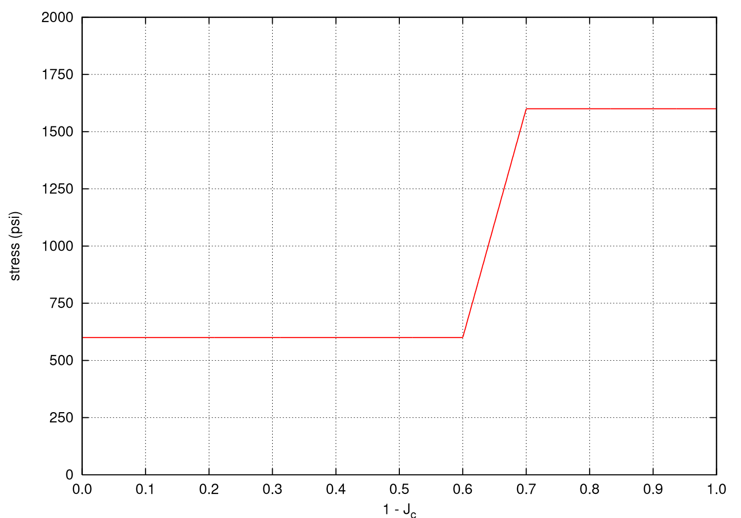
Fig. 4.131 An example of an input crush curve for an aluminum honeycomb.

Above some value of compaction (\(1-J_c=V_{min}\)), the material will be fully compacted and behave as an elastic, perfectly plastic material. The fully compacted response is given by the Young’s modulus, \(E\), Poisson’s ratio, \(\nu\), and the yield stress, \(\sigma_{y}\). Details of this response may be found in previous sections on the various elastic-plastic models (e.g. Section 4.7.1).

4.30.2. Implementation

Implementation of the orthotropic crush model involves addressing two cases: before and after complete compaction. When the material is fully crushed, the model reduces to that of an isotropic perfectly plastic response. As corresponding isotropic elastic-plastic models with various hardenings have been extensively explored in prior sections, this response will not be discussed here and the reader is referred to those sections (e.g. Section 4.7.2). The two cases are distinguished by the previous compaction state variable, \(J_c^{n}\), where \(J_c^{n+1}=\min\left[J_c^n,J^{n+1}\right]\) with \(J^{n+1}=\det\left(F_{ij}^{n+1}\right)=\det\left(V_{ij}^{n+1}\right)\). If \(J_c^{n}>1-V_{min}\), the material has not yet fully crushed and the response is evaluated as discussed in the following.

To determine the material state prior to complete compaction, the current values of orthogonal stiffness must be determined via (4.143) noting

\[\alpha^{n+1}=\frac{1-J_c^{n}}{V_{min}}.\]

By assuming completely elastic deformation, trial stresses may then be computed as,

\[\begin{split}\sigma^{tr}_{11} & = \sigma^n_{11}+\Delta t\hat{E}_{11}\left(\alpha^{n+1}\right)d^{n+1}_{11}, \nonumber \\ \sigma^{tr}_{22} & = \sigma^n_{22}+\Delta t\hat{E}_{22}\left(\alpha^{n+1}\right)d^{n+1}_{22}, \nonumber \\ \sigma^{tr}_{33} & = \sigma^n_{33}+\Delta t\hat{E}_{33}\left(\alpha^{n+1}\right)d^{n+1}_{33}, \\ \sigma^{tr}_{12} & = \sigma^n_{12}+2\Delta t\hat{G}_{12}\left(\alpha^{n+1}\right)d^{n+1}_{12}, \nonumber \\ \sigma^{tr}_{23} & = \sigma^n_{23}+2\Delta t\hat{G}_{23}\left(\alpha^{n+1}\right)d^{n+1}_{23}, \nonumber \\ \sigma^{tr}_{31} & = \sigma^n_{31}+2\Delta t\hat{G}_{31}\left(\alpha^{n+1}\right)d^{n+1}_{31}, \nonumber\end{split}\]

with \(d_{ij}^{n+1}\) being the unrotated rate of deformation tensor. Given the decoupling between the different stress components, the various trial stresses are considered individually. Specifically, each trial stress must be compared to the crush stress for the current compaction level. Denoting \(\sigma^{crush}_{\beta}=\hat{\sigma}_{\beta}\left(1-J_c^{n+1}\right)\) (with \(\beta= 11,~22,~33,~12,~23,\) or \(31\)) to be the current crush stress specified by the crush curve, the current stress of interest is,

\[\begin{split}\sigma_{\beta}^{n+1} = \left\{\begin{array}{cc}\sigma^{tr}_{\beta}, & |\sigma^{tr}_{\beta}| \leq \sigma^{crush}_{\beta} \\ \text{sgn}\left(\sigma^{tr}_{\beta}\right) \sigma^{crush}_{\beta}, & |\sigma^{tr}_{\beta}| > \sigma^{crush}_{\beta}, \end{array}\right.\end{split}\]

where \(\text{sgn}\left(x\right)\) returns the sign of the argument and is used as \(\sigma^{crush}_{\beta}\) is entered as a positive number.

4.30.3. Verification

The orthotropic crush model was verified through a series of uniaxial compression tests. Given the lack of coupling between the different directions, such a variety of tests were performed to test each loading component. One set of material properties was used for all tests and they are given in Table 4.47.

Table 4.47 The material properties for the orthotropic crush model used for the uniaxial crush tests.

\(E_{11}\)	50.0 ksi	\(E\)	1000.0 ksi
\(E_{22}\)	220.0 ksi	\(\nu\)	0.25
\(E_{33}\)	10.0 ksi	\(\sigma_y\)	2.0 ksi
\(G_{12}\)	110.0 ksi
\(G_{23}\)	5.0 ksi	\(V_{min}\)	0.7
\(G_{31}\)	25.0 ksi

The crush curves used as input for these tests are given in Fig. 4.132.

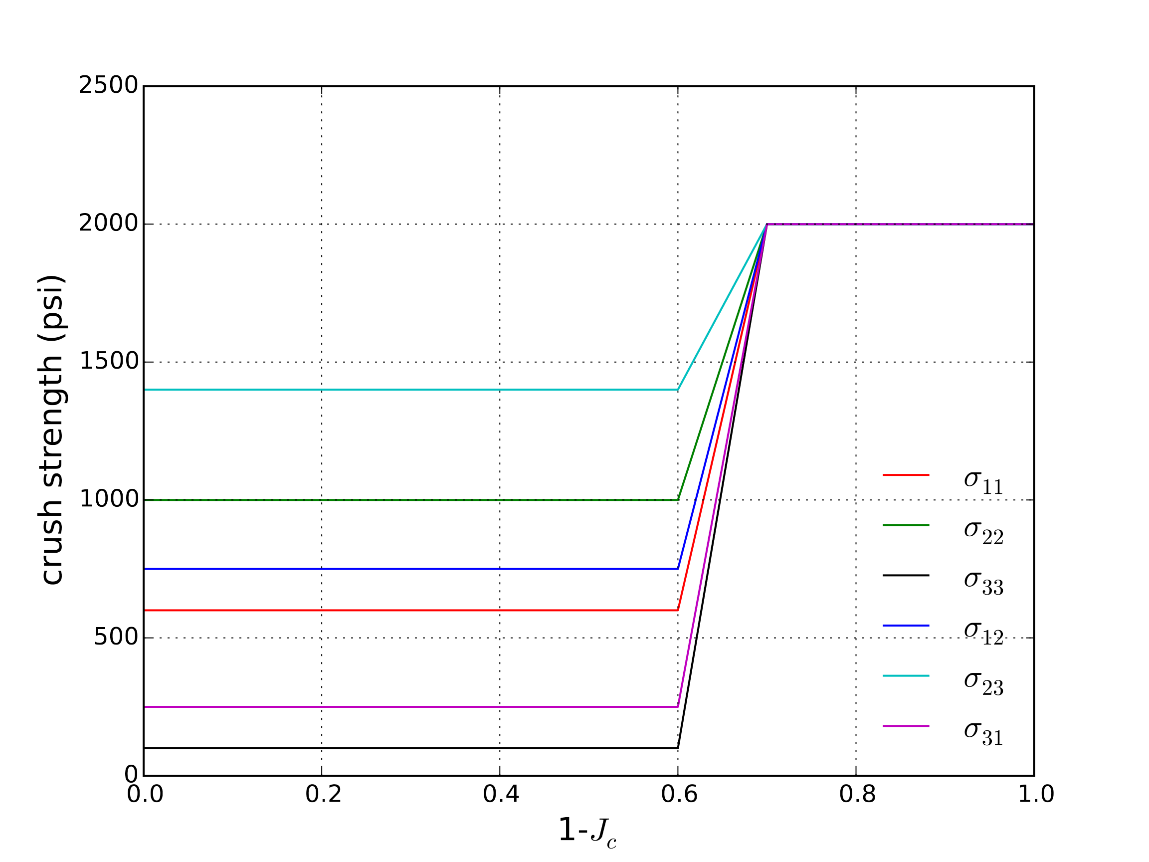
Fig. 4.132 Input crush curves used for uniaxial crush analysis.

To test this model, both the anisotropic nature and different deformation regimes need to be tested. Therefore, given the decoupled directional nature prior to complete compaction, each component will be tested. For the diagonal stress components, a simple uniaxial displacement of the form,

\[u_{i}=-\lambda\delta_{i\beta},\]

where \(\beta=1,~2,\) or \(3\) corresponding to the directional component being tested is applied. In such cases (with a monotonically increasing \(\lambda\)), \(J_c = 1-\lambda\). The model described in the prior to sections can be easily evaluated analytically under such conditions, and the corresponding analytical and numerical results are presented in Fig. 4.133.

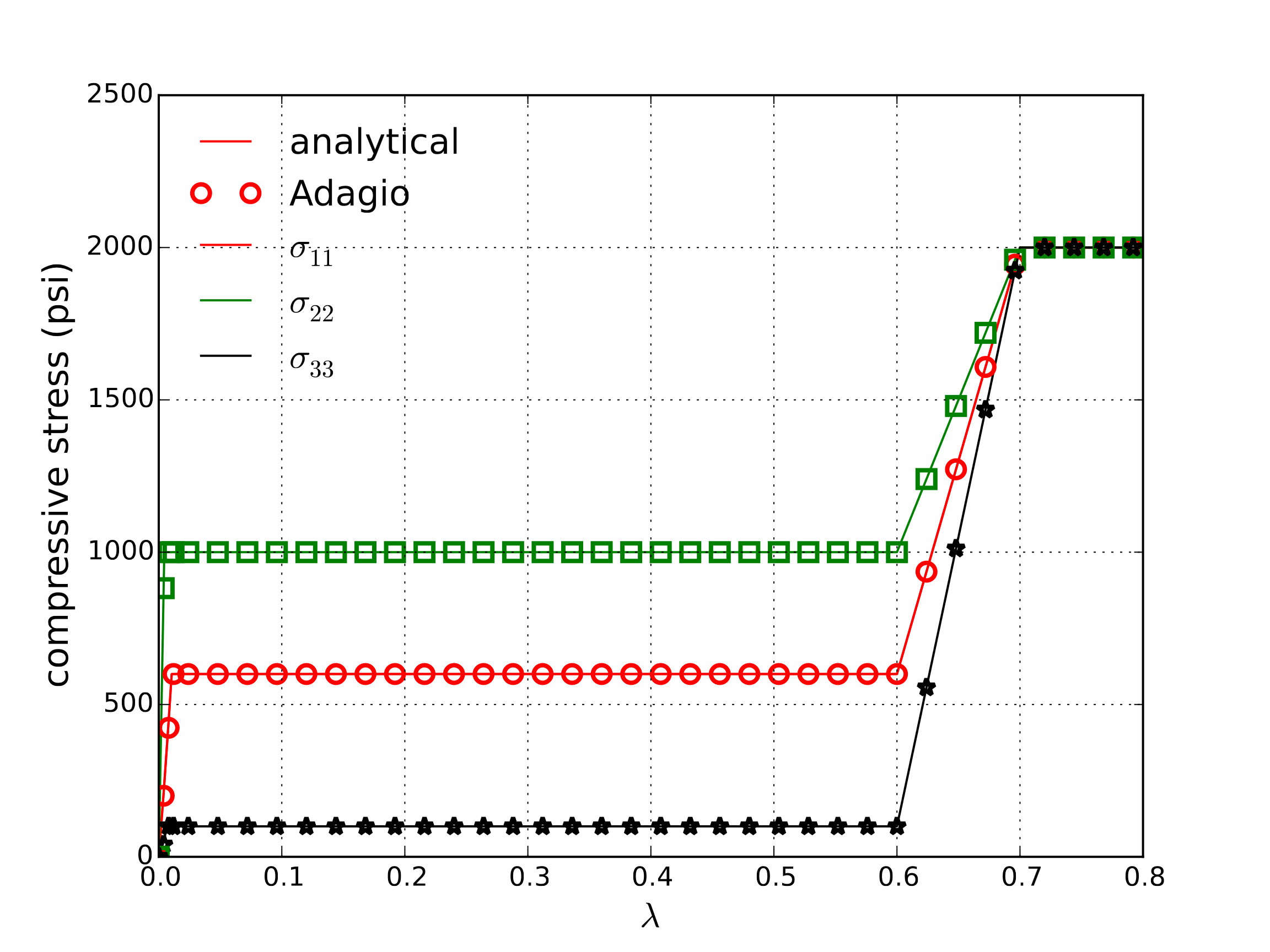
Fig. 4.133 Analytical and numerical results for uniaxial crush cases.

4.30.4. User Guide

BEGIN PARAMETERS FOR MODEL ORTHOTROPIC_CRUSH
  #
  # Elastic constants - Post lock-up
  YOUNGS MODULUS = <real>
  POISSONS RATIO = <real>
  SHEAR MODULUS  = <real>
  BULK MODULUS   = <real>
  LAMBDA         = <real>
  TWO MU         = <real>
  #
  # Orthotropic Elastic properties - Pre-Crush
  #
  EX             = <real>
  EY             = <real>
  EZ             = <real>
  GXY            = <real>
  GYZ            = <real>
  GZX            = <real>
  #
  # Crush properties
  #
  CRUSH XX       = <string>
  CRUSH YY       = <string>
  CRUSH ZZ       = <string>
  CRUSH XY       = <string>
  CRUSH YZ       = <string>
  CRUSH ZX       = <string>
  VMIN           = <real>
  #
  # Post lock-up yield properties
  #
  YIELD STRESS   = <real>
  #
END [PARAMETERS FOR MODEL ORTHOTROPIC_CRUSH]

In the above command blocks:

• The EX, EY, EZ, GXY, GYZ, and GZX command lines define, respectively, the initial, pre-crush directional moduli \(E_{xx}\), \(E_{yy}\), \(E_{zz}\), \(G_{xy}\), \(G_{yz}\), and \(G_{zx}\) from (4.142).

• CRUSH XX, YY, ZZ, XY, YZ, and ZX inputs require the name of a function defined via a FUNCTION command line in the SIERRA scope. These functions describe the directional crush characteristics of the material and give the current stress value (in a direction) as a function of the current compaction (\(1-J_c\)).

• The command VMIN defines the minimum relative volume of the material that is achieved when the material is completely crushed. This parameter may also be considered as the maximum compaction.

• The elastic constant commands refer to the post lock-up, fully compacted isotropic response of the material.

• YIELD STRESS refers to the plateau stress of the material after lock-up when the response is perfectly plastic.

Output variables available for this model are listed in Table 4.48. For information about the orthotropic crush model, consult [[1]].

Table 4.48 State Variables for ORTHOTROPIC CRUSH Model

Name	Description
CRUSH	current (unrecoverable) compaction/relative volume

---

[1] (1,2)

R.G. Whirley, B.E. Engelmann, and J.O. Halquist. DYNA3D user’s manual. 1991.