4.14. Hosford Plasticity Model

4.14.1. Theory

Like other elastic-plastic models in LAMÉ, the Hosford plasticity model is a rate-independent hypoelastic formulation. Unlike the Hill and other more complex plasticity models, it is isotropic. In a similar fashion to those models, the total rate of deformation is additively decomposed into an elastic and plastic part such that

\[D_{ij}=D^{\text{e}}_{ij}+D^{\text{p}}_{ij}.\]

The objective stress rate, depending only on the elastic deformation, may then be written as,

\[\stackrel{\circ}{\sigma}_{ij}=\mathbb{C}_{ijkl}D^{\text{e}}_{kl}.\]

The Hosford plasticity model utilizes a yield surface first put forth by W. F. Hosford in the 1970’s [[1]] that is isotropic but non-quadratic. This specific form was proposed due to experimental observations of biaxial stretching in which neither the Tresca or \(J_2\) yield surfaces could describe the results. In contrast to many of the yield surfaces proposed for similar purposes, only two parameters are utilized. Even with these limited terms, the developed model is quite versatile and can be reduced to von Mises or Tresca conditions as well as capturing responses in between. This yield surface is given as,

\[f\left(\sigma_{ij},\bar{\varepsilon}^p\right)=\phi\left(\sigma_{ij}\right)-\bar{\sigma}\left(\bar{\varepsilon}^p\right)=0,\]

in which \(\phi\left(\sigma_{ij}\right)\) is the Hosford effective stress and \(\bar{\sigma}\left(\bar{\varepsilon}^p\right)\) is the current yield stress that may depend on rate and/or temperature. The Hosford effective stress is a non-quadratic function of the principal stresses (\(\sigma_i,~~i=1,2,3\)) and is given as

\[\phi\left(\sigma_{ij}\right)=\left[\frac{|\sigma_1-\sigma_2|^a+|\sigma_2-\sigma_3|^a+|\sigma_1-\sigma_3|^a}{2}\right]^{1/a}\]

in which \(a\) is the yield surface exponent. Interestingly, if \(a=2\) or \(4\) the yield surface reduces to that of a \(J_2\) von Mises surface while \(a=1\) or as \(a\rightarrow\infty\) produces a Tresca like shape. If the value of \(a\) is above 4 the yield surface takes a position between the Tresca and \(J_2\) limits. Typical values are \(a=6\) or \(a=8\) for bcc and fcc metals, respectively [[2]]. To highlight this variability the yield surface is plotted below in Fig. 4.46 for three values of \(a\) – \(a~=~4,~8,\) and 100.

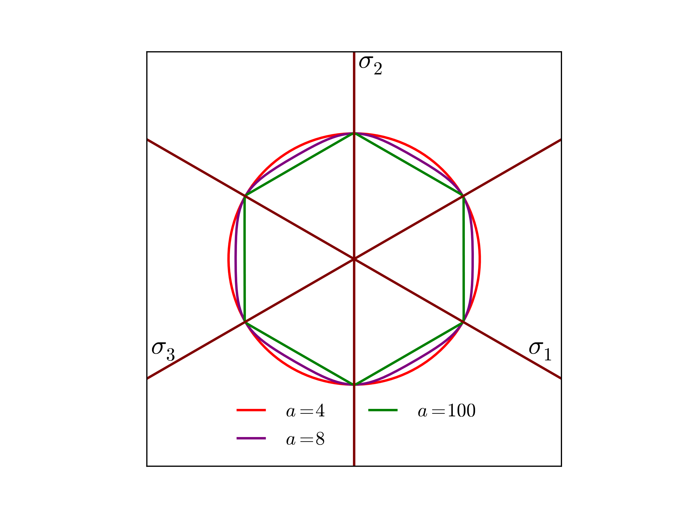
Fig. 4.46 Example Hosford yield surfaces, \(f\left(\sigma_{ij},\bar{\varepsilon}^p=0;a\right)\), presented in the deviatoric \(\pi\)-plane. The presented surfaces correspond to the different yield exponents \(a~=~4,~8,\) and \(100\).

For the hardening function, \(\bar{\sigma}\left(\bar{\varepsilon}^p\right)\), a variety of forms including linear, power law, or a more general user defined function may be used.

An associated flow rule is utilized such that the plastic rate of deformation is normal to the yield surface and is given by,

\[\dot{D}_{ij}^{\text{p}}=\dot{\gamma}\frac{\partial\phi}{\partial\sigma_{ij}},\]

where \(\dot{\gamma}\) is the consistency multiplier enforcing \(f=0\) during plastic deformation. Given the form of \(f\), it can also be shown that \(\dot{\gamma}=\dot{\bar{\varepsilon}}^p\).

For details on the plasticity model, please see [[3]]. Additional details on failure models and adiabatic heating capabilities may be found in [[4], [5]] and [[6]], respectively.

4.14.1.1. Plastic Hardening

Plastic hardening refers to increases in the flow stress, \(\bar{\sigma}\), with plastic deformation. As such, hardening is described via a functional relationship between the flow stress and isotropic hardening variable (effective plastic strain), \(\bar{\sigma}\left(\bar{\varepsilon}^p\right)\). Over the course of nearly a century of work in metal plasticity, a variety of relationships have been proposed to describe the interactions associated with different physical interpretations, deformation mechanisms, and materials. To enable the utilization of the same plasticity models for different material systems, a modular implementation of plastic hardening has been adopted such that the analyst may select different hardening models from the input deck thereby avoiding any code changes or user subroutines. In this section, additional details are given for the different models to enable the user to select the appropriate choice of model. Note, the models being discussed here are only for isotropic hardening in which the yield surface expands. Kinematic hardening in which the yield surface translates in stress-space with deformation and distortional hardening where the shape of the yield surface changes shape with deformation are not treated. For a larger discussion of the phenomenology and history of different hardening types, the reader is referred to [[7], [8], [9]].

Given the ubiquitous nature of these hardening laws in computational plasticity, some (if not most) of this material may be found elsewhere in this manual. Nonetheless, the discussion is repeated here for the convenience of the reader.

4.14.1.1.1. Linear

Linear hardening is conceptually the simplest model available in LAMÉ. As the name implies, a linear relationship is assumed between the hardening variable, \(\bar{\varepsilon}^p\), and flow stress. The hardening modulus, \(H^{\prime}\), is a constant giving the rate of change of flow stress with plastic flow. The flow stress expression may therefore be written,

\[\bar{\sigma}=\sigma_y + H^{\prime}\bar{\varepsilon}^p.\]

The simplicity of the model is its main feature as the constant slope,

\[\frac{d\bar{\sigma}}{d\bar{\varepsilon}^p}=H^{\prime},\]

makes the model attractive for analytical models and cheap for computational implementations (e.g. radial return algorithms require only a single correction step). Unfortunately, the simplicity of the representation also means that it has limited predictive capabilities and can lead to overly stiff responses.

4.14.1.1.2. Power Law

Another common expression for isotropic hardening is the power-law hardening model. Due to its prevalence, a dedicated ELASTIC-PLASTIC POWER LAW HARDENING model may be found in LAMÉ (see Section 4.8.1). This expression is given as,

\[\bar{\sigma}=\sigma_y + A<\bar{\varepsilon}^p-\varepsilon_L>^n,\]

in which \(<\cdot>\) are Macaulay brackets, \(\varepsilon_L\) is the Luders strain, \(A\) is a fitting constant, and \(n\) is an exponent typically taken such that \(0<n\leq1\). The Luders strain is a positive, constant strain value (defaulted to zero) giving an initially perfectly plastic response in the plastic deformation domain (see Fig. 4.20). The derivative is then simply,

\[\frac{d\bar{\sigma}}{d\bar{\varepsilon}^p}=nA<\bar{\varepsilon}^p-\varepsilon_L>^{\left(n-1\right)}.\]

Note, one difficulty in such an implementation is that when the effective equivalent plastic strain is zero, numerical difficulties may arise in evaluating the derivative and necessitate special treatment of the case.

4.14.1.1.3. Voce

The Voce hardening model (sometimes referred to as a saturation model) uses a decaying exponential function of the equivalent plastic strain such that the hardening eventually saturates to a specified value (thus the name). Such a relationship has been observed in some structural metals giving rise to the popularity of the model. The hardening response is given as,

\[\bar{\sigma}=\sigma_y + A\left(1-\exp\left(-n\bar{\varepsilon}^p\right)\right),\]

in which \(A\) is a fitting constant and \(n\) is a fitting exponent controlling how quickly the hardening saturates. Importantly, the derivative is written as,

\[\frac{d\bar{\sigma}}{d\bar{\varepsilon}^p}=nA\exp\left(-n\bar{\varepsilon}^p\right),\]

and is well defined everywhere giving the selected form an advantage over the aforementioned power law model.

4.14.1.1.4. Johnson-Cook

The Johnson-Cook hardening model is a variant of the classical Johnson-Cook [[10], [11]] expression. In this instance, the temperature-dependence is neglected to focus on the rate-dependent capabilities while allowing for arbitrary isotropic hardening forms via the use of a user-defined hardening function. With these assumptions, the flow stress may be written as,

\[\bar{\sigma}=\tilde{\sigma}_y\left(\bar{\varepsilon}^p\right)\left[1+C\left<\ln\left(\frac{\dot{\bar{\varepsilon}}^p}{\dot{\varepsilon}_0}\right)\right>\right],\]

in which \(\tilde{\sigma}_y\left(\bar{\varepsilon}^p\right)\) is the user-specified rate-independent hardening function, \(C\) is a fitting constant and \(\dot{\varepsilon}_0\) is a reference strain rate. The Macaulay brackets ensure the material behaves in a rate independent fashion when \(\dot{\bar{\varepsilon}}^p < \dot{\varepsilon}_0\).

4.14.1.1.5. Power Law Breakdown

Like the Johnson-Cook formulation, the power-law breakdown model is also rate-dependent. Again, a multiplicative decomposition is assumed between isotropic hardening and the corresponding rate-dependence dependent. In this case, however, the functional form is derived from the analysis of Frost and Ashby [[12]] in which power-law relationships like those of the Johnson-Cook model cease to appropriately capture the physical response. The form used here is similar to the expression used by Brown and Bammann [[13]] and is written as,

\[\bar{\sigma} = \tilde{\sigma}_y\left(\bar{\varepsilon}^p\right)\left[1+\text{asinh}\left(\left(\frac{\dot{\bar{\varepsilon}}^p}{g}\right)^{\left(1/m\right)}\right)\right],\]

with \(\tilde{\sigma}_y\left(\bar{\varepsilon}^p\right)\) being the user supplied rate independent expression, \(g\) is a model parameter related to the activation energy required to transition from climb to glide-controlled deformation, and \(m\) dictates the strength of the dependence.

4.14.2. Implementation

The Hosford plasticity model is implicitly integrated using a closest point projection (CPP) return mapping algorithm (RMA). The resulting nonlinear equations are solved via a line search augmented Newton-Raphson method and the stress update routine is very similar to that of the Hill plasticity model. The key difference between the two is the isotropy. Specifically, given that the Hosford yield surface is isotropic and the functional form is given in terms of principal stresses, the stress update routine is performed in principal stress space and then converted to global Cartesian values.

For a loading step, a trial stress state, \(T^{tr}_{ij}\), may be computed by knowing the rate of deformation, \(d_{ij}\), and time step as,

\[T_{ij}^{tr}=T_{ij}^n+\Delta t\mathbb{C}_{ijkl}d_{kl}.\]

The principal stresses, \(T_{i}^{tr}\), may then be used to determine the trial yield function value, \(\phi^{tr}=\phi\left(T_i^{tr}, \bar{\varepsilon}^{p\left(n\right)}\right)\). If \(\phi^{tr}<0\), the elastic trial solution is acceptable. On the other hand, if the trial solution is inadmissible, the aforementioned CPP-RMA problem is solved in principal stress space. The crux of this algorithm is the simultaneous solution of two nonlinear equations – (i) the flow rule and (ii) consistency condition. The former leads to a residual, \(R_i\), of the form (again in principal stress space),

\[R_{i}=\Delta d^p_{i}-\Delta \gamma\frac{\partial\phi}{\partial T_{i}}=0,\]

while the latter is enforced by the yield function,

\[f=\phi\left(T_i\right)-\bar{\sigma}\left(\bar{\varepsilon}^p\right)=0,\]

and its derivative (\(\dot{f}\)) being zero. This system is solved via a Newton-Raphson type approach in which the state variables (stress, \(T_{i}\), and consistency multiplier, \(\gamma\)) are iteratively corrected until the residuals are satisfied. Using \(\left(k+1\right)\) and \(\left(k\right)\) to denote the next and current iterations, this updating takes the form,

(4.45)\[\begin{split}\Delta \gamma^{\left(k+1\right)} & = \Delta \gamma^{\left(k\right)}+\Delta\left(\Delta\gamma\right), \nonumber \\ T_{i}^{\left(k+1\right)} & = T_{i}^{\left(k\right)}+\Delta T_{i},\end{split}\]

in which \(T^{\left(0\right)}=T_i^{tr}\) and \(\Delta \gamma^{\left(0\right)}=0\). Consistent linearization of the two equations can be solved to give correction increments of the form,

\[\begin{split}\Delta\left(\Delta\gamma\right) & = \frac{f^{\left(k\right)}-R^{\left(k\right)}_i\mathcal{L}_{ij}^{\left(k\right)} \frac{\partial\phi^{\left(k\right)}}{\partial T_j}}{\frac{\partial\phi^{\left(k\right)}}{\partial T_i} \mathcal{L}_{ij}^{\left(k\right)}\frac{\partial\phi^{\left(k\right)}}{\partial T_j}+H^{'\left(k\right)}} ,\nonumber \\ \Delta T_i & = -\mathcal{L}_{ij}^{\left(k\right)}\left(R_j^{\left(k\right)}+\Delta\left(\Delta\gamma\right)\frac{\partial\phi^{\left(k\right)}} {\partial T_j}\right),\end{split}\]

with \(\mathcal{L}_{ij}^{\left(k\right)}\) being the Hessian of the CPP-RMA problem and \(H^{'\left(k\right)}\) is the slope of the hardening curve.

Previous studies have indicated that the Newton-Raphson method alone may be insufficient to guarantee convergence with arbitrary stress states in the case of non-quadratic yield surfaces [[14], [15], [3]]. To address this, a line search method is adopted. In such an approach, the incrementation rule (4.45) is modified such that,

(4.46)\[\begin{split}\Delta \gamma^{\left(k+1\right)} & = \Delta \gamma^{\left(k\right)}+\alpha\Delta\left(\Delta\gamma\right), \nonumber \\ T_{i}^{\left(k+1\right)} & = T_{i}^{\left(k\right)}+\alpha\Delta T_{i},\end{split}\]

where \(\alpha\in\left(0,1\right]\) is the step magnitude. This parameter enforces that the solution be converging and is determined via various convergence criteria. The \(\alpha=1\) case corresponds to the Newton-Raphson method. Utilization of this approach has been shown to greatly increase the robustness of this algorithm under large trial stresses [[3]].

Finally, upon convergence of the algorithm, the Cartesian stress are found from the principal stresses via,

\[T_{ij}^{n+1}=\sum_{k=1}^3T_k^{n+1}\hat{e}_i^k\hat{e}_j^k,\]

in which \(\hat{e}_i^k\) is the eigenvector of the \(k^{th}\) principal stress.

Details of this implementation and the line search algorithm may be found in the work of Scherzinger [[3]].

4.14.3. Verification

The Hosford plasticity material model is verified through a variety of loading and material conditions. For these cases, the elastic properties corresponding to 2090-T3 aluminum [[16]] given in Section 4.15.3 are utilized. Additional verification exercises for the various failure models and adiabatic heating capabilities may be found in [[4], [5]] and [[6]], respectively.

The elastic properties are \(E=70\) GPa and \(\nu = 0.25\) while a linear hardening law of the form,

\[\bar{\sigma}\left(\bar{\varepsilon}^p\right) = \sigma_{y} + K\bar{\varepsilon}^p,\]

with \(\sigma_{y}=200\) MPa and \(K=E/200\) is assumed. For these studies, two different yield surface exponents will be used, \(a=4,~8\). The former corresponds to the \(J_2\) surface while the latter is a common value for aluminum.

4.14.3.1. Uniaxial Stress

In the case of uniaxial stress (\(\sigma\)), it is trivial to note that the corresponding principal stress state is simply \(\sigma_1=\sigma,~\sigma_2=\sigma_3=0\). As such, regardless of \(a\),

\[\phi=|\sigma_1|.\]

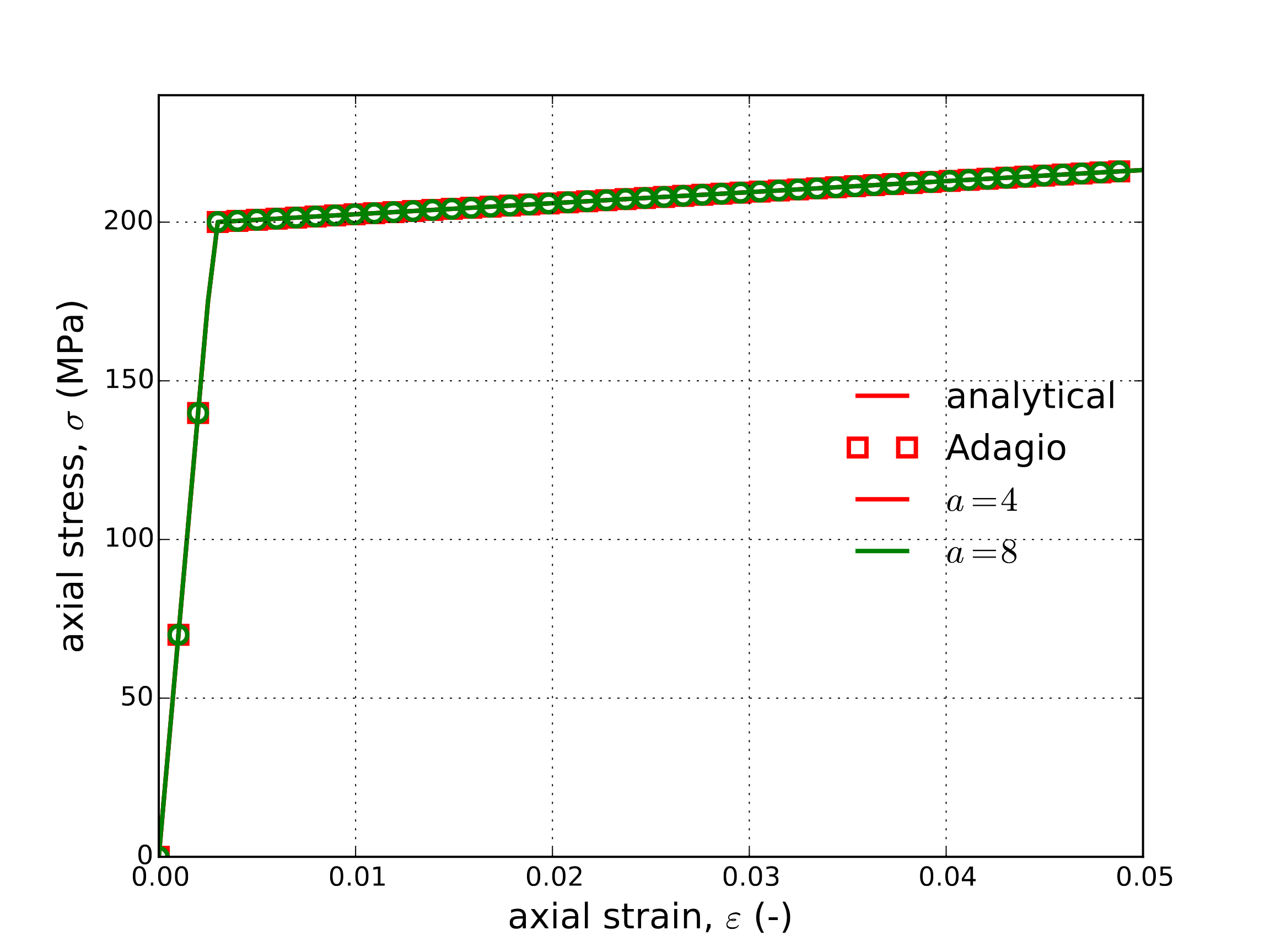
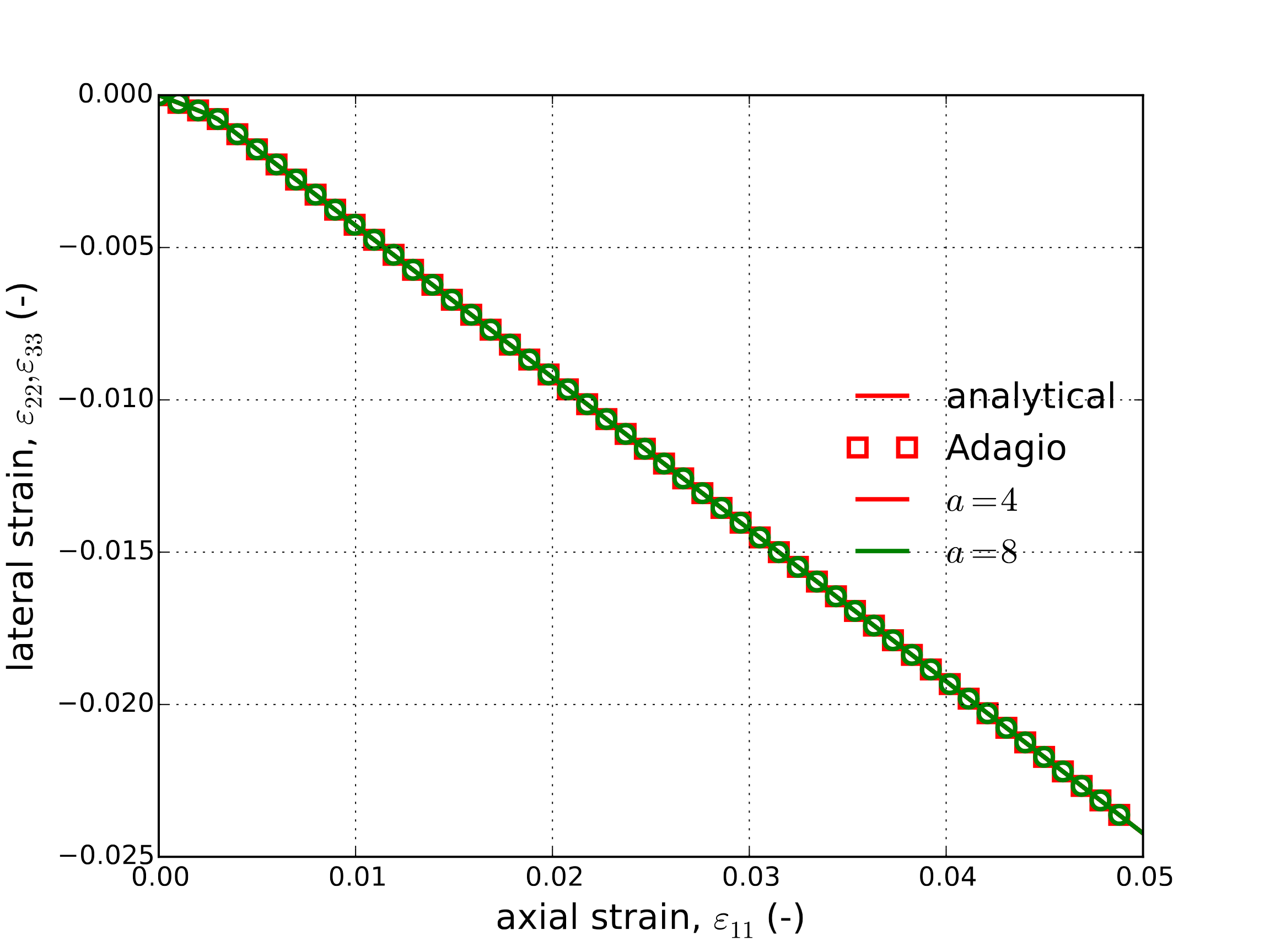
With the aforementioned linear hardening, this case reduces to that discussed in Section 4.7.3.1. Corresponding analytical and numerical results (both with \(a=4\) and \(8\)) of the axial stress and lateral strain are presented in Fig. 4.47(a) and Fig. 4.47(b), respectively. In these figures, the invariance of response on yield surface exponent through this loading is clearly observed.

Uniaxial Stress

Lateral Strain

Fig. 4.47 Axial stress-strain (a) and lateral strain (b) results of the Hosford plasticity model determined analytically and numerically for the case of yield surface exponents \(a=4,8\).

4.14.3.2. Pure Shear

To explore the impact of the yield exponent \(a\), the case of pure shear is considered. Specifically, the only shear component shall be in the Cartesian \(e_1-e_2\) direction such that \(\sigma_{12}=\tau\) and \(\varepsilon_{12}\) are the only non-zero components. Noting that the three principal stresses are \(\tau,0,-\tau\), the yield condition simplifies to

\[\phi=\left[1+2^{a-1}\right]^{1/a}\tau.\]

The equivalent plastic strain may then be found as a function of \(\varepsilon_{12}\) in the same way as presented in Section 4.15.3.2. Shear stress-strain results for both \(a=4,~8\) are presented in Fig. 4.48 as determined both by adagio and analytically. The boundary conditions for this loading are given in Appendix A. In these results, the effect of the yield surface exponent, \(a\), may clearly be seen.

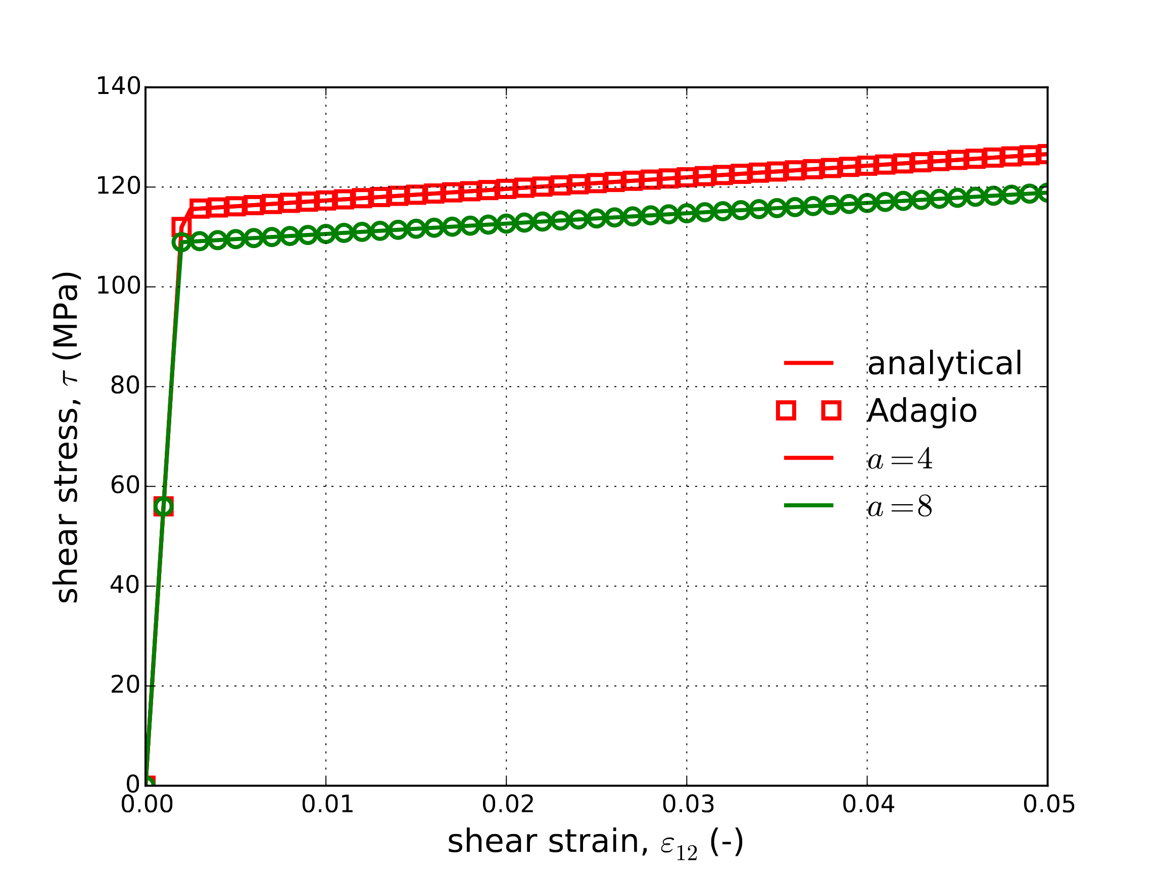
Fig. 4.48 Shear stress-strain results of the Hosford plasticity model determined analytically and numerically for the case of yield surface exponents \(a=4,~8\).

4.14.3.3. Plastic Hardening

To verify the capabilities of the hardening models, rate independent and rate dependent alike, the constant equivalent plastic strain rate, \(\dot{\bar{\varepsilon}}^p\), uniaxial stress and pure shear verification tests described in Appendix A are utilized. In these simplified loading cases, the material state may be found explicitly as a function of time knowing the prescribed equivalent strain rate. For the rate independent cases, a strain rate of \(\dot{\bar{\varepsilon}}^p=1\times10^{-4} \text{s}^{-1}\) is used for ease in simulations although the selected rate does not affect the results. Through this testing protocol, the hardening models are not only tested at different rates but also different yield surface shapes. In the current Hosford case, multiple yield surface exponents, \(a\), are considered to probe this effect. Additionally, the rate dependent models are tested for a wide range of strain rates (over five decades) and with all three rate independent hardening functions (\(\tilde{\sigma}_y\) in the previous theory section). Although linear, Voce, and power-law rate independent representations are utilized in the rate dependent tests, in those cases the hardening models are prescribed via user-defined analytic functions. The rate independent verification exercises, on the other hand, examine the built-in hardening models. This distinction necessitates the different considerations and treatments.

The various rate dependent and rate independent hardening coefficients are found in Table 4.18 while the remaining model parameters are unchanged from the previous verification exercises. For the current verification exercises, the rate independent hardening models (linear, Voce, and power-law) will first be considered and then the rate dependent forms (Johnson-Cook, power-law breakdown).

Table 4.18 The model parameters for the hardening verification tests used with the Hosford plasticity model during verification tests. Parameters for the rate independent hardening functions, \(\tilde{\sigma}_y\), are also given and denoted with a \(\tilde{\cdot}\) while the subscript refers to the functional form.

\(C\)	0.1	\(\dot{\varepsilon}_0\)	\(1\times 10^{-4}\) s\(^{-1}\)
\(g\)	0.21 s\(^{-1}\)	\(m\)	16.4
\(\tilde{H}_{\text{Linear}}\)	200 MPa
\(\tilde{A}_{\text{PL}}\)	400 MPa	\(\tilde{n}_{\text{PL}}\)	0.25
\(\tilde{A}_{\text{Voce}}\)	200 MPa	\(\tilde{n}_{\text{Voce}}\)	20

4.14.3.3.1. Linear

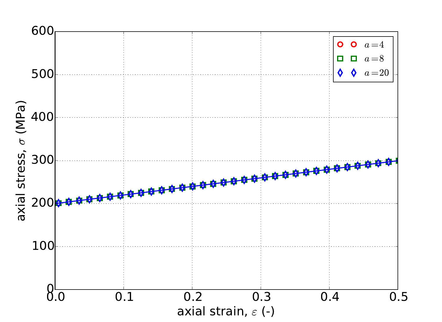
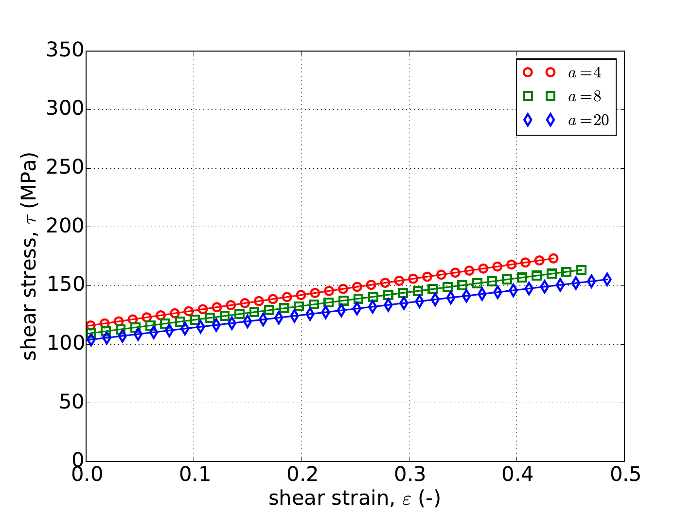
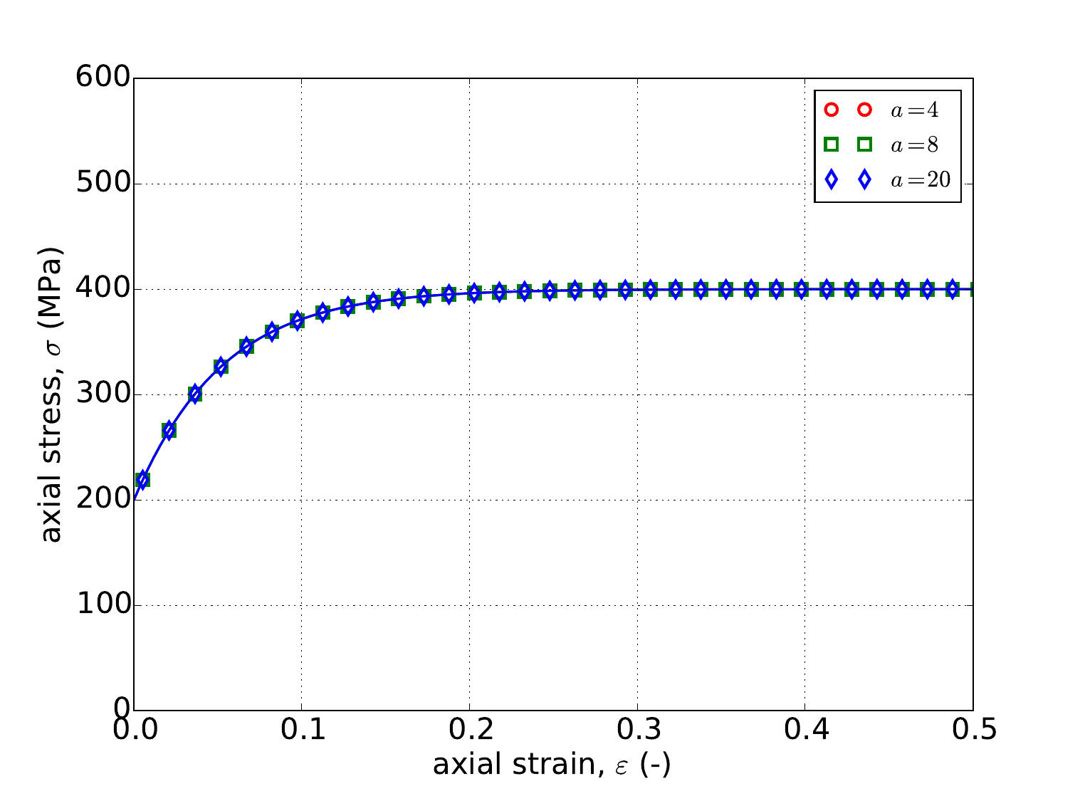
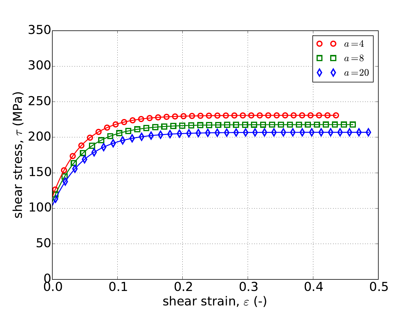
The aforementioned verification exercises from Appendix A are used to investigate the numerical implementation of the rate independent linear hardening model. Results from uniaxial stress and pure shear exercises determined analytically and numerically are given in Fig. 4.49 for three different exponents \(a=~4,~8,\) and \(20\). The first exponent produces a \(J_2\) like response with the latter increasing the curvature of the yield surface. As discussed in Section 4.14.3.1, a purely uniaxial response is independent of exponent thus producing the collapsed results in Fig. 4.49. In both the uniaxial stress and pure shear cases, clear agreement is noted between the two sets of results. The linear slope (tangent modulus) giving the model its name is also observable in the results of Fig. 4.49.

Uniaxial Stress

Pure Shear

Fig. 4.49 Uniaxial stress-strain (a) and pure shear (b) responses of the Hosford plasticity model with rate independent, linear hardening. Solid line are analytical while open symbols are numerical.

4.14.3.3.2. Power-Law

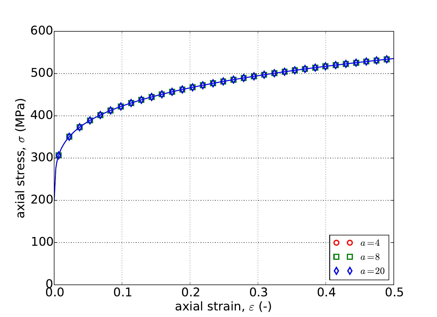
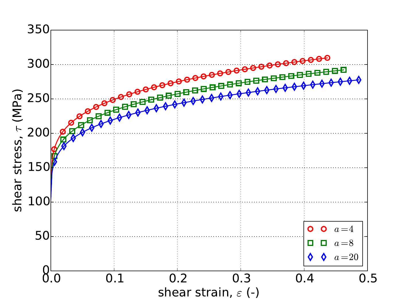
To consider the performance of the common power-law hardening model with the Hosford yield surface, the uniaxial stress and pure shear exercises of Appendix A are solved analytically and numerically. These results are presented in Fig. 4.50 for three different Hosford exponents – \(a=~4,~8\) and \(20\). As expected from previous discussions the uniaxial stress results in Fig. 4.50(a) are independent of \(a\). For both the uniaxial stress and pure shear results, the desired agreement between analytical and numerical solutions is apparent. These results also highlight the initial curved response during plastic-deformation eventually transitioning into a more linear type response.

Uniaxial Stress

Pure Shear

Fig. 4.50 Uniaxial stress-strain (a) and pure shear (b) responses of the Hosford plasticity model with rate independent, power-law hardening. Solid line are analytical while open symbols are numerical.

4.14.3.3.3. Voce

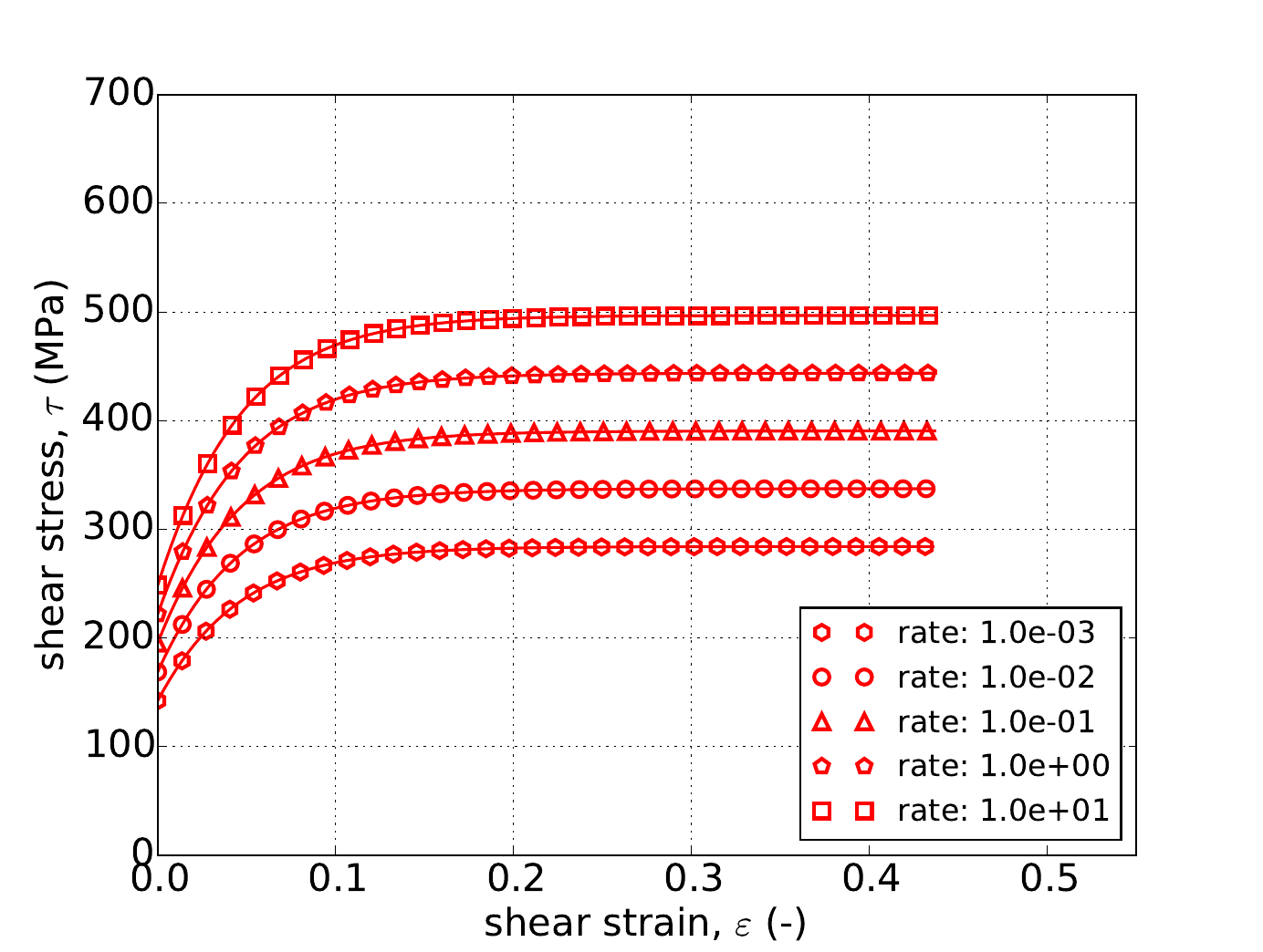
For the rate independent Voce hardening model, the problems of Appendix A are used to verify the model response. Specifically, results for the uniaxial stress and pure shear analyses are presented in Fig. 4.51 as determined analytically and numerically for three different values of \(a\) – \(a=~4,~8,\) and \(20\). From these results, clear agreement is noted between the two sets of results; including the invariance of the uniaxial stress case to \(a\) (Fig. 4.51a). Additionally, the results of Fig. 4.51 also exemplify the saturation nature of the Voce hardening model as the stress-strain response eventually asymptotes.

Uniaxial Stress

Pure Shear

Fig. 4.51 Uniaxial stress-strain (a) and pure shear (b) responses of the Hosford plasticity model with rate independent, Voce hardening. Solid line are analytical while open symbols are numerical.

4.14.3.3.4. Johnson-Cook

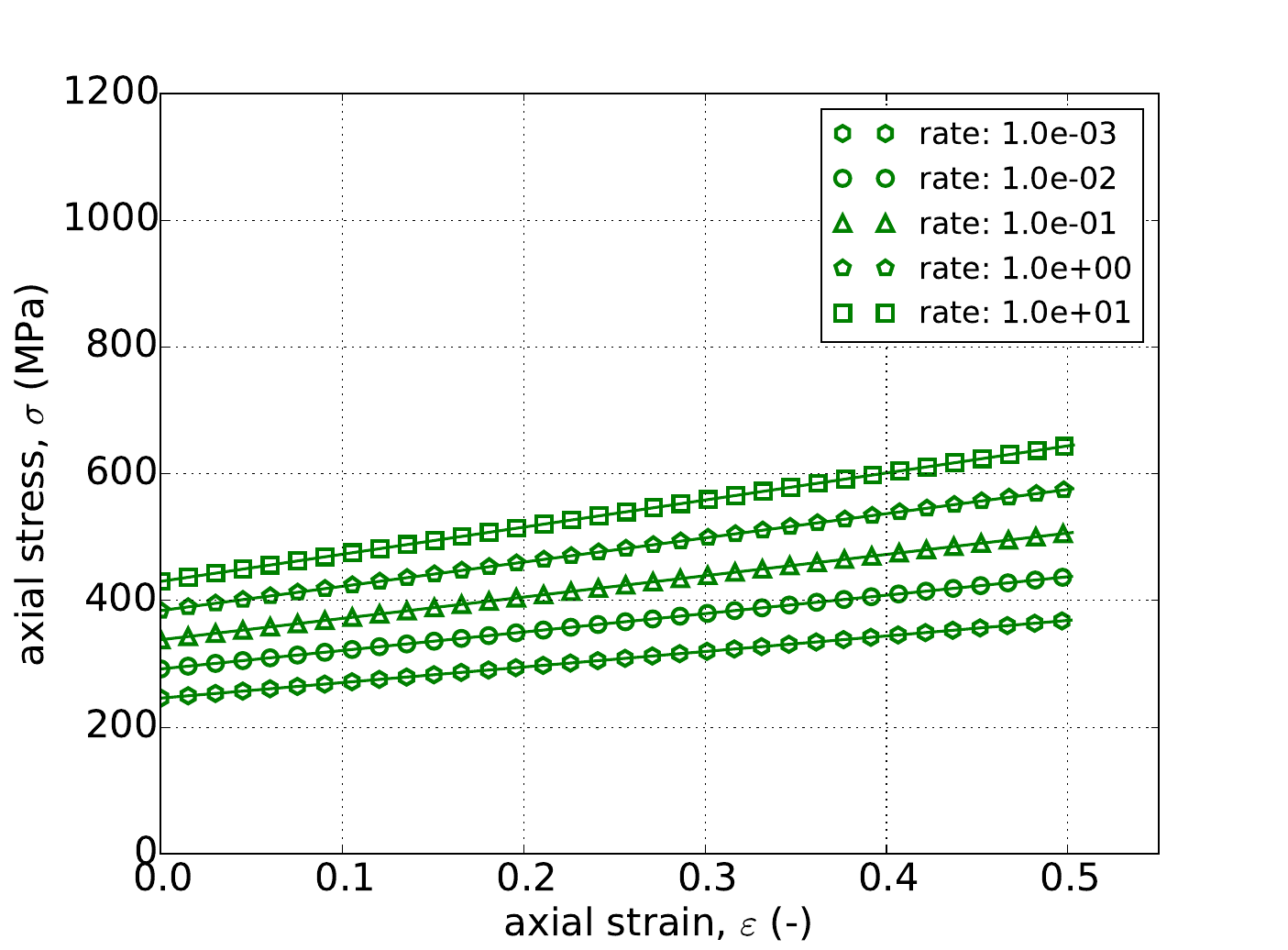
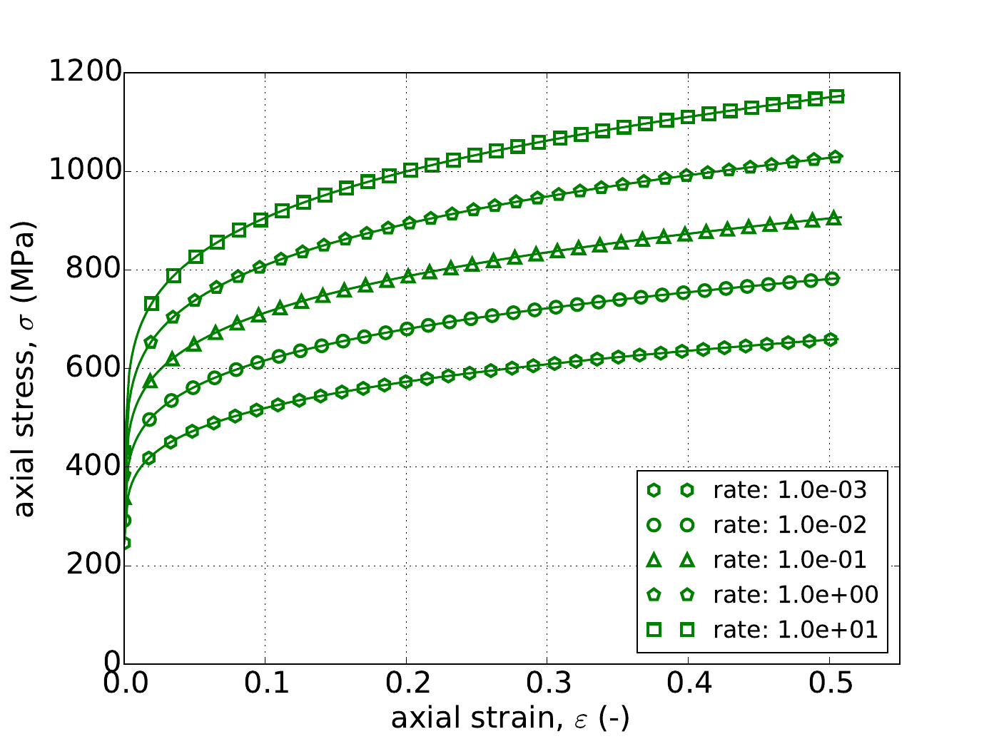
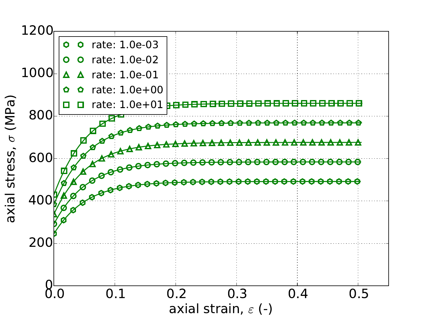
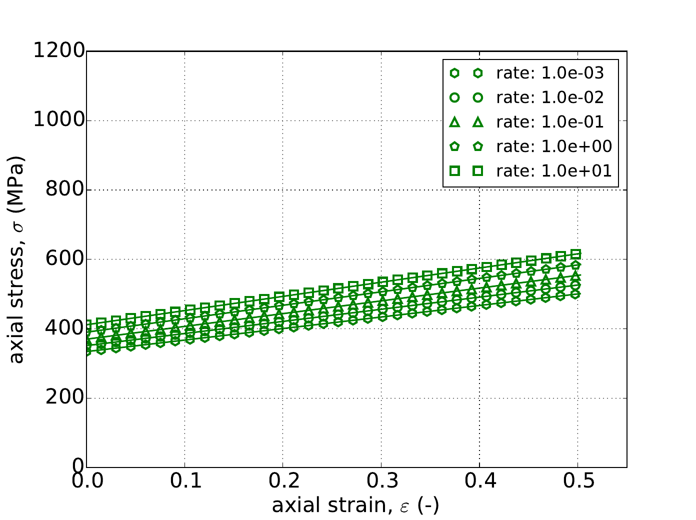
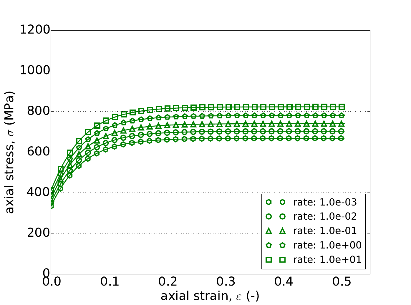
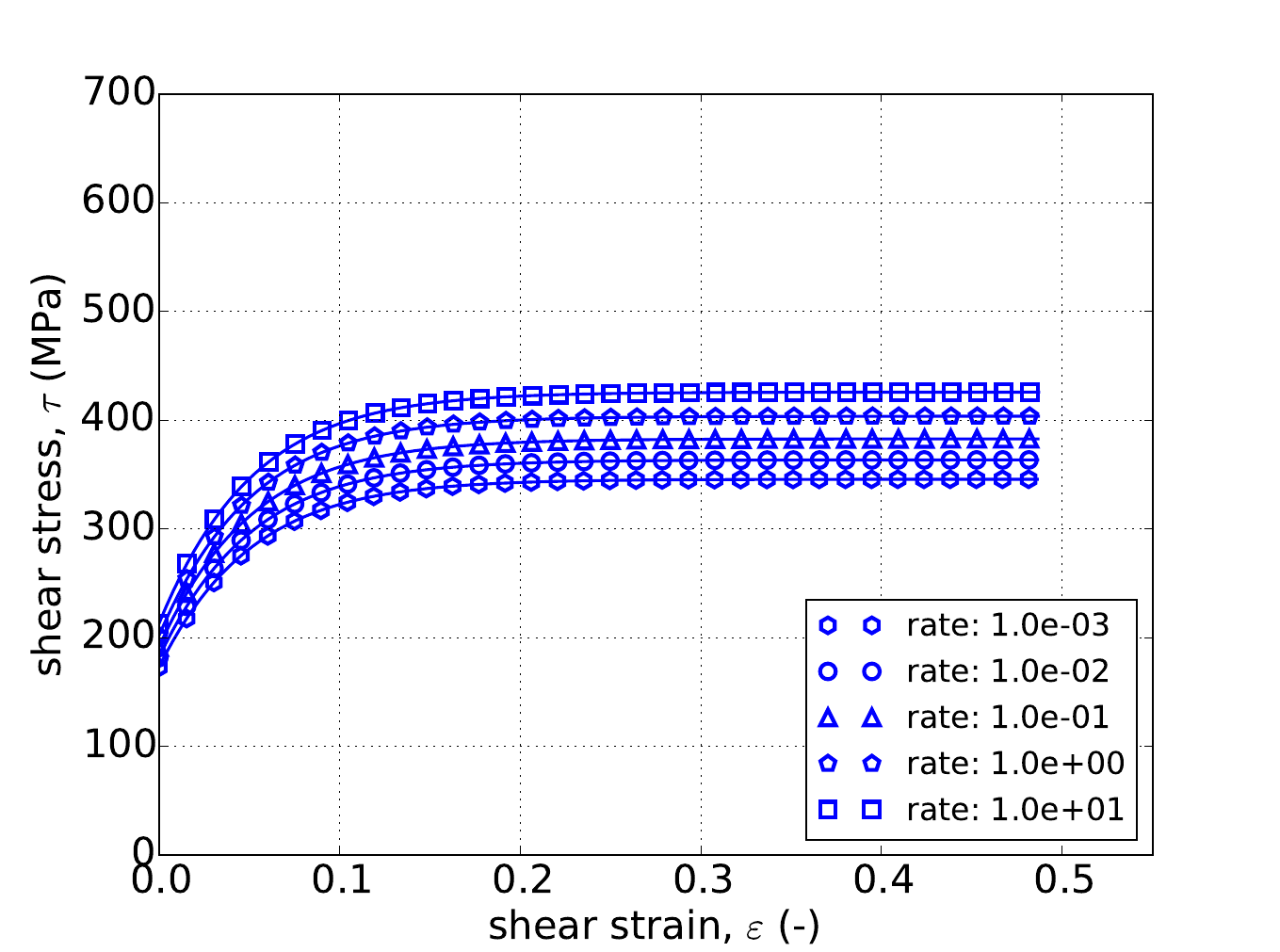
As noted in Section 4.14.3.1, the uniaxial stress response is independent of \(a\). This is also reflected Appendix A in which the stress weighting coefficients (\(\Gamma\)) for the Hosford uniaxial case are one. As such in Fig. 4.52 the results of the constant equivalent plastic strain rate uniaxial stress test are presented with \(a=8\) and using the linear (Fig. 4.52a), power-law (Fig. 4.52b), and Voce (Fig. 4.52c) rate independent hardening models for five different rates – \(\dot{\bar{\varepsilon}}^p=1\times10^{-3},~1\times10^{-2},~1\times10^{-1},~1\times10^{0}\) and \(1\times10^{1}~\text{s}^{-1}\). In all cases in Fig. 4.52 excellent agreement is observed between the results.

Linear Hardening

Power-Law Hardening

Voce Hardening

Fig. 4.52 Uniaxial stress-strain response of the Hosford plasticity model (\(a=8\)) with rate dependent, Johnson-Cook type hardening with (a) linear (b) power-law and (c) Voce rate independent hardening. Solid lines are analytical results while open symbols are numerical.

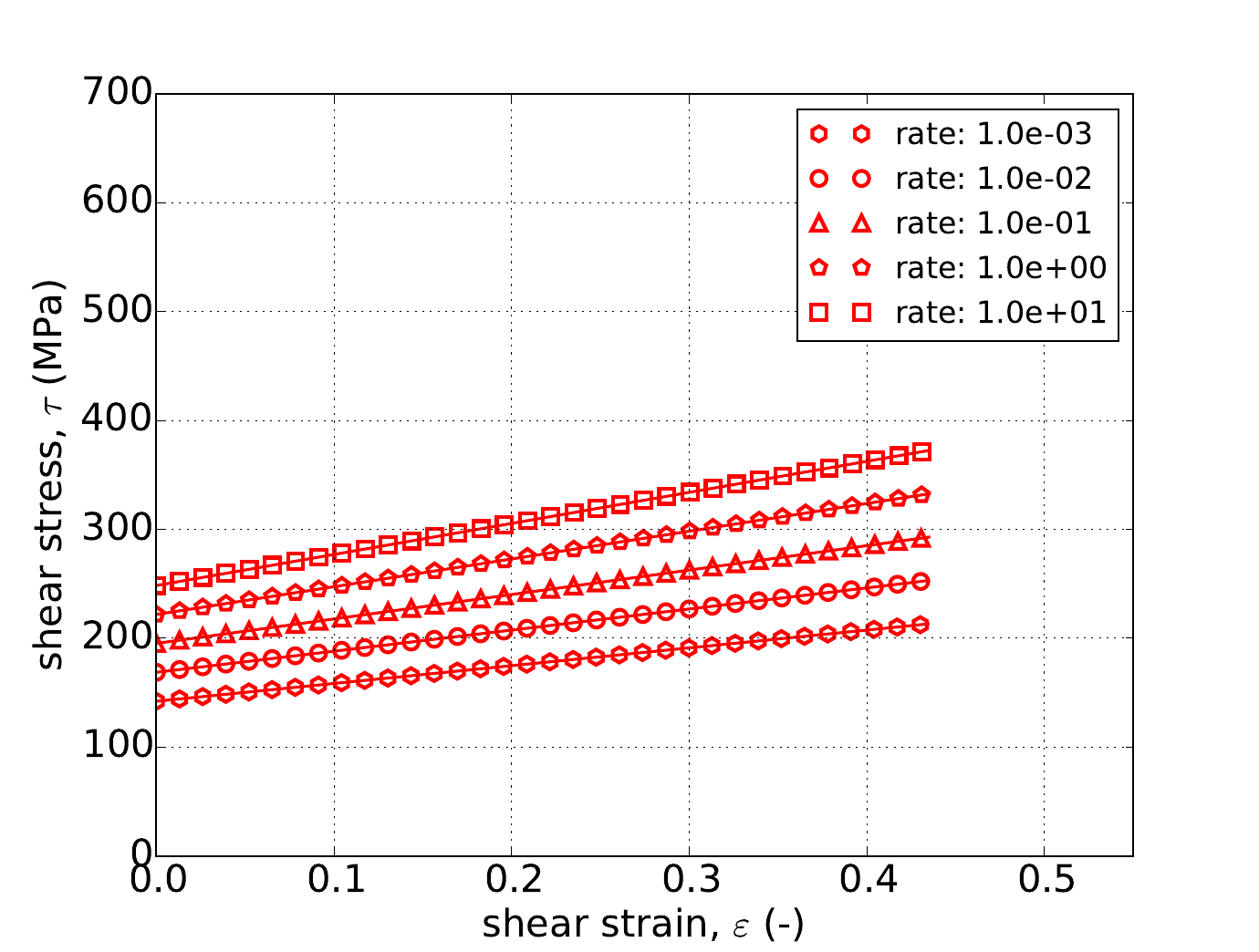
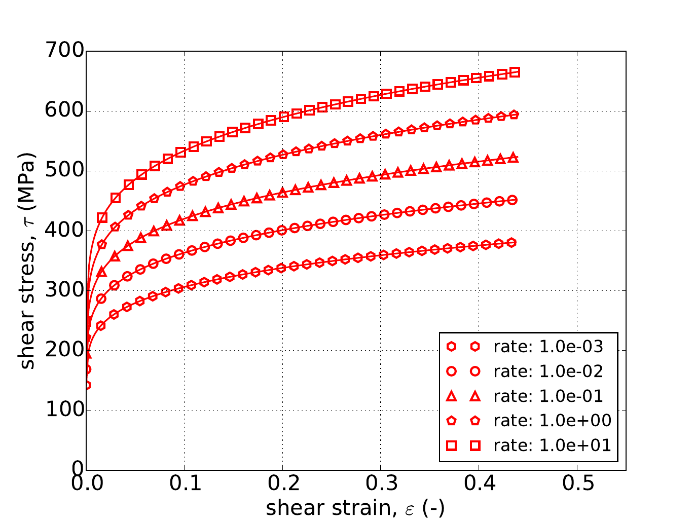
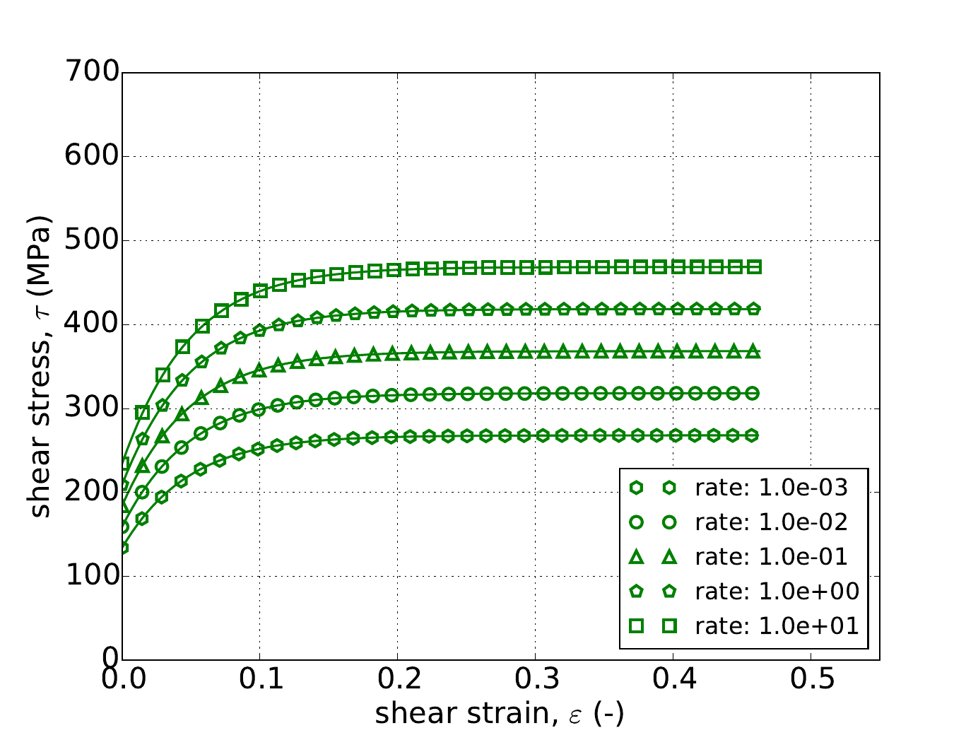
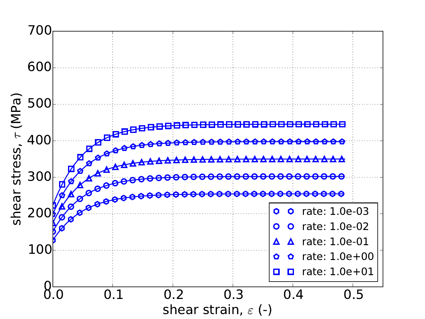
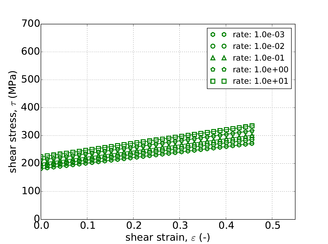
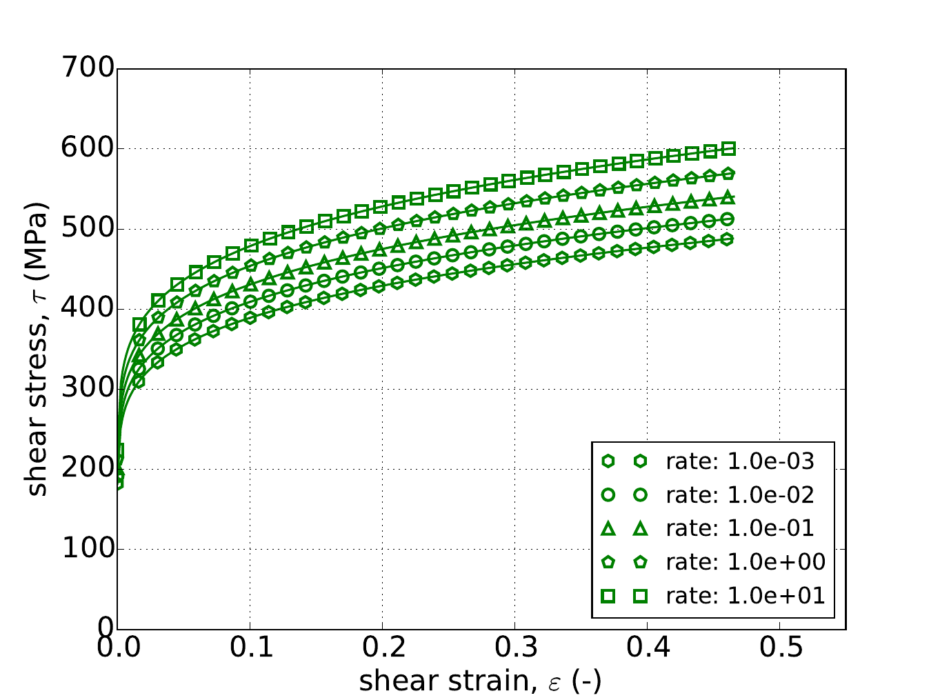
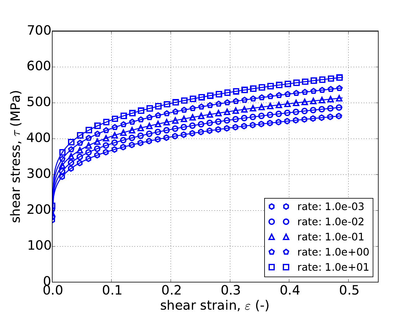
Unlike the uniaxial stress case, for pure shear the response depends on the exponent \(a\). Therefore, in addition to the three hardening models, results are also presented for three different exponent values – \(a=4,~8,\) and \(20\). The results for all nine cases are presented in Fig. 4.53 and Fig. 4.54 and again excellent agreement is noted in all instances.

Linear Hardening a=4

Linear Hardening, a=8

Linear Hardening, a=20

Power-Law Hardening, a=4

Power-Law Hardening, a=8

Power-Law Hardening, a=20

Fig. 4.53 Stress-strain response of the Hosford plasticity model with rate dependent, Johnson-Cook type hardening in pure shear with (a-c) linear (d-f) and power-law rate independent hardening. Solid lines are analytical results while open symbols are numerical.

Power-Law Hardening, a=4

Power-Law Hardening, a=8

Power-Law Hardening, a=20

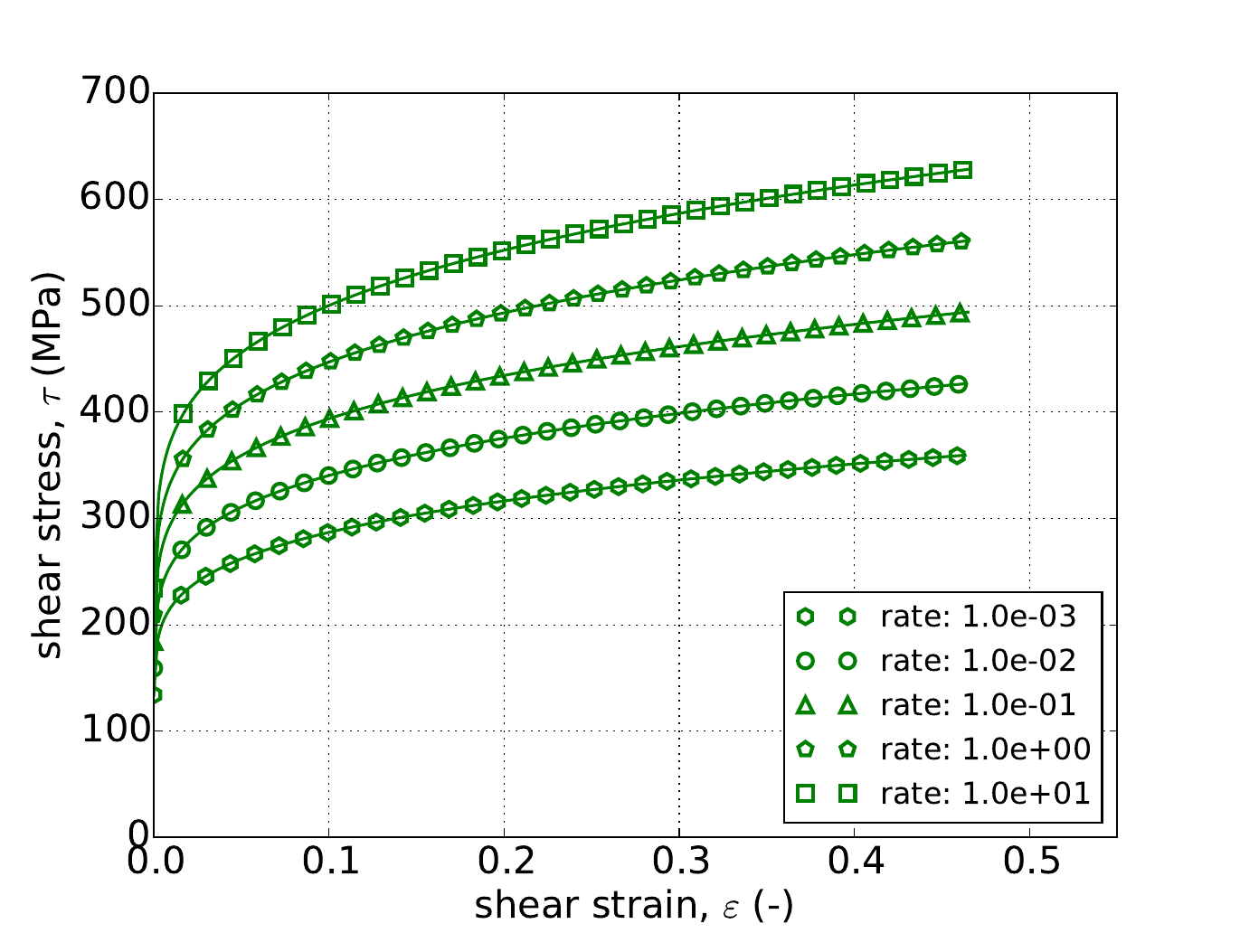
Fig. 4.54 Stress-strain response of the Hosford plasticity model with rate dependent, Johnson-Cook type hardening in pure shear with (a-c) Voce rate independent hardening. Solid lines are analytical results while open symbols are numerical.

4.14.3.3.5. Power-Law Breakdown

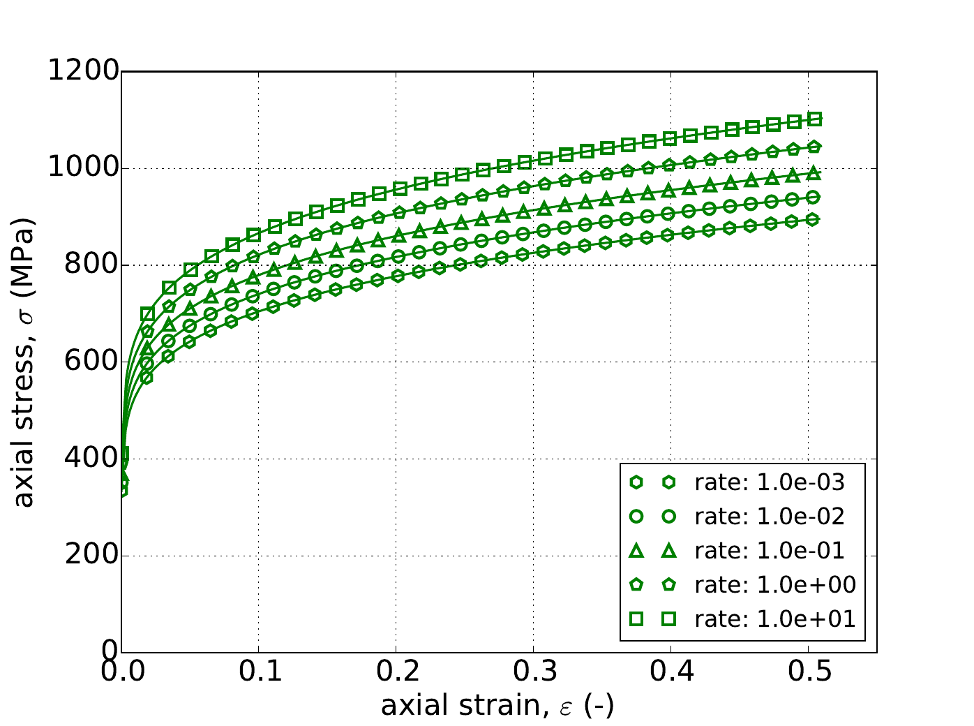
As mentioned in the previous Johnson-Cook section, for the Hosford model under uniaxial stress the response is independent of yield surface exponent, \(a\). Therefore, Fig. 4.55 presents the results of the constant equivalent plastic strain rate verification test of Appendix A for strain rates spanning five decades – \(\dot{\bar{\varepsilon}}^p=1\times10^{-3},~1\times10^{-2},~1\times10^{-1},~1\times10^{0}\) and \(1\times10^{1}~\text{s}^{-1}\). The tests are performed for each rate- independent hardening model. In all fifteen cases excellent agreement is noted between numerical and analytical results.

Linear Hardening

Power-Law Hardening

Voce Hardening

Fig. 4.55 Uniaxial stress-strain response of the Hosford plasticity model (\(a=8\)) with rate dependent, power-law breakdown type hardening with (a) linear (b) power-law and (c) Voce rate independent hardening. Solid lines are analytical results while open symbols are numerical.

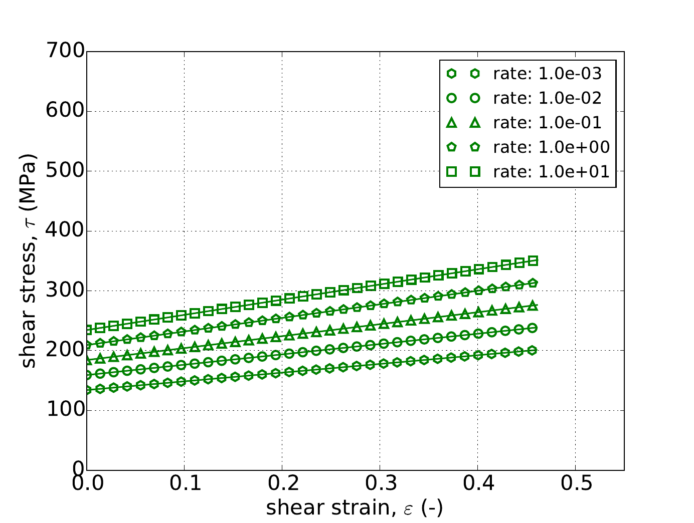
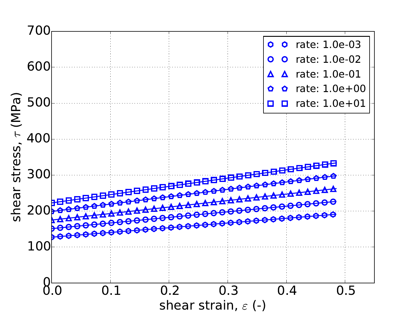
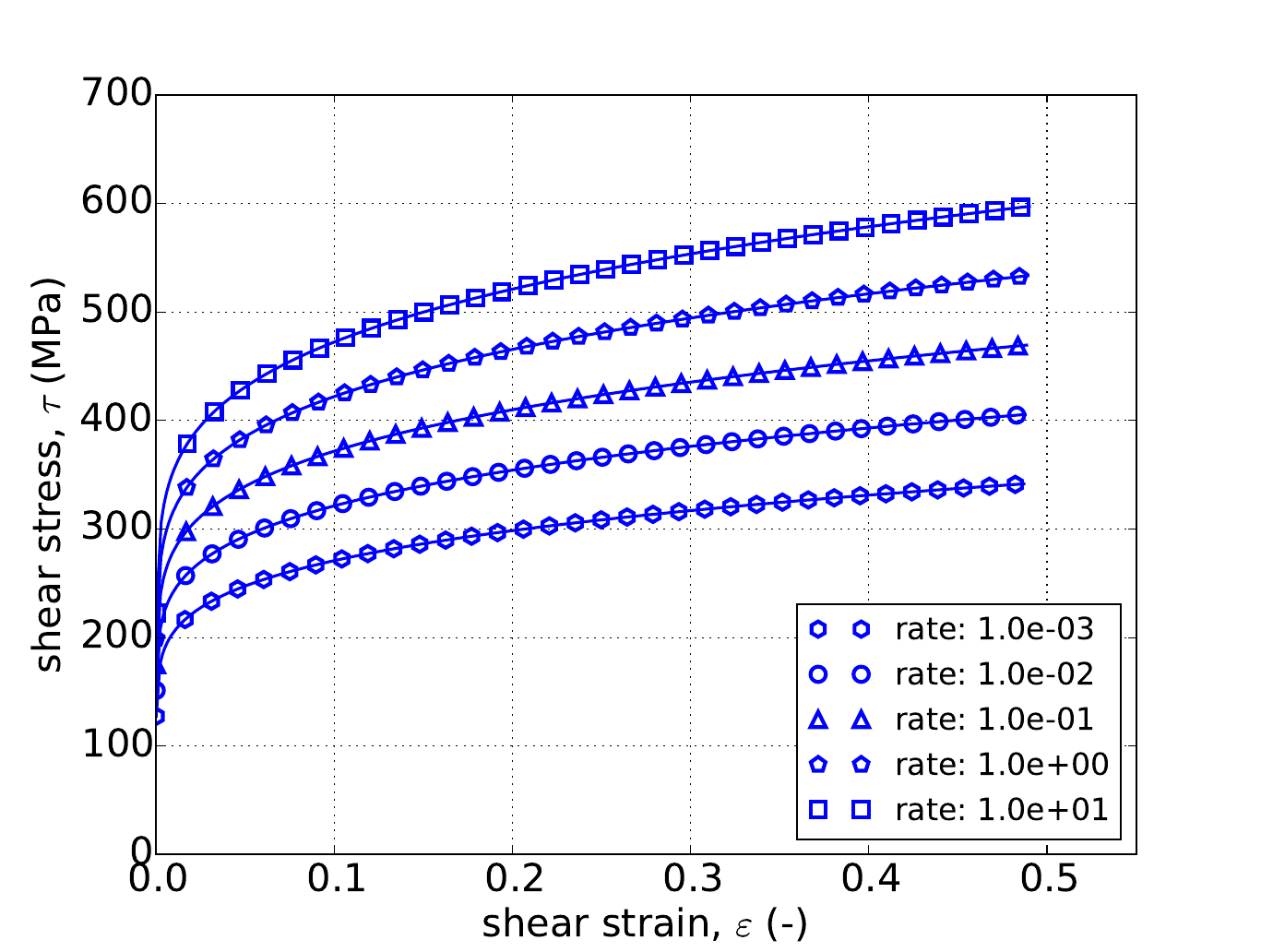
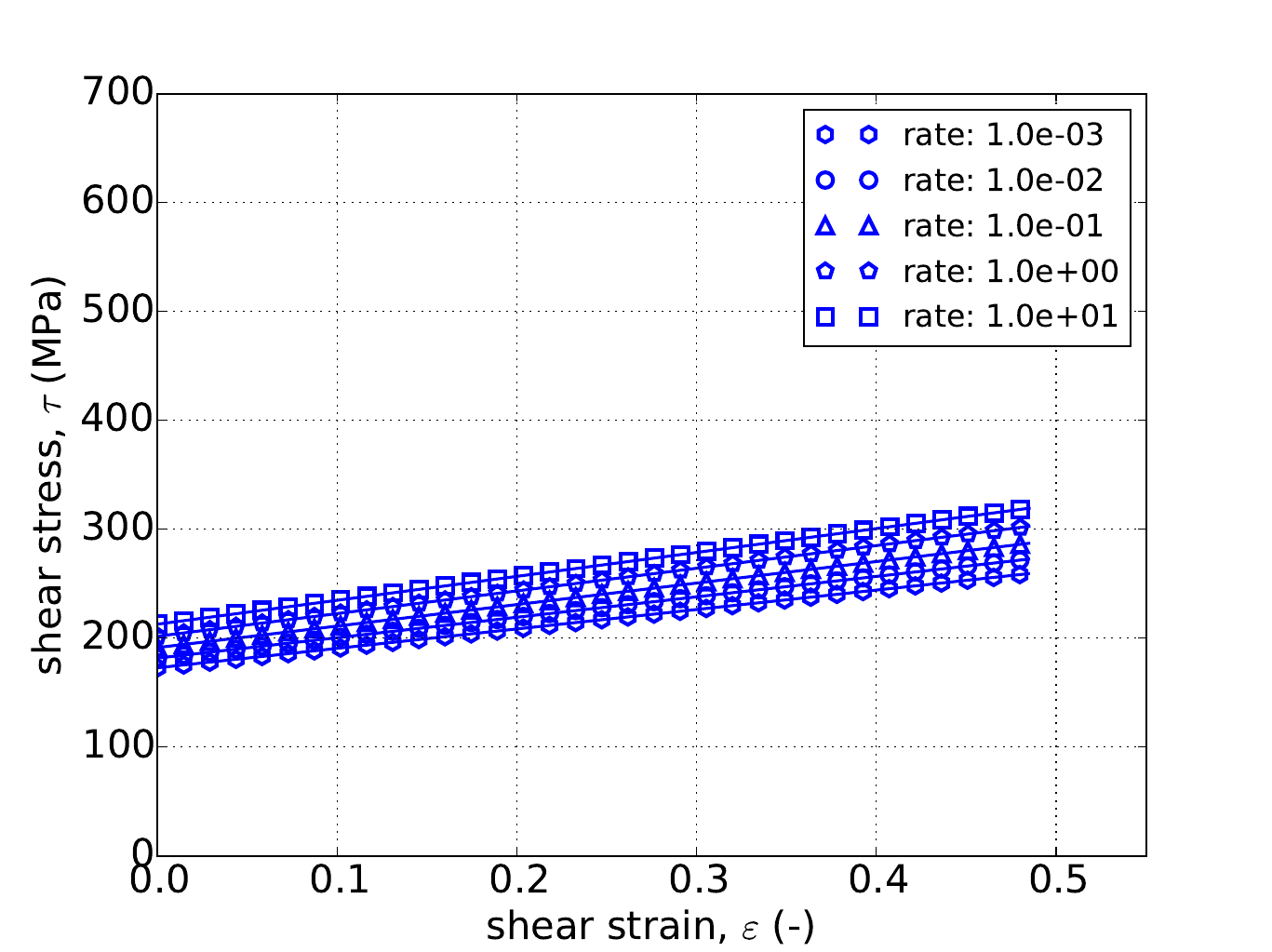
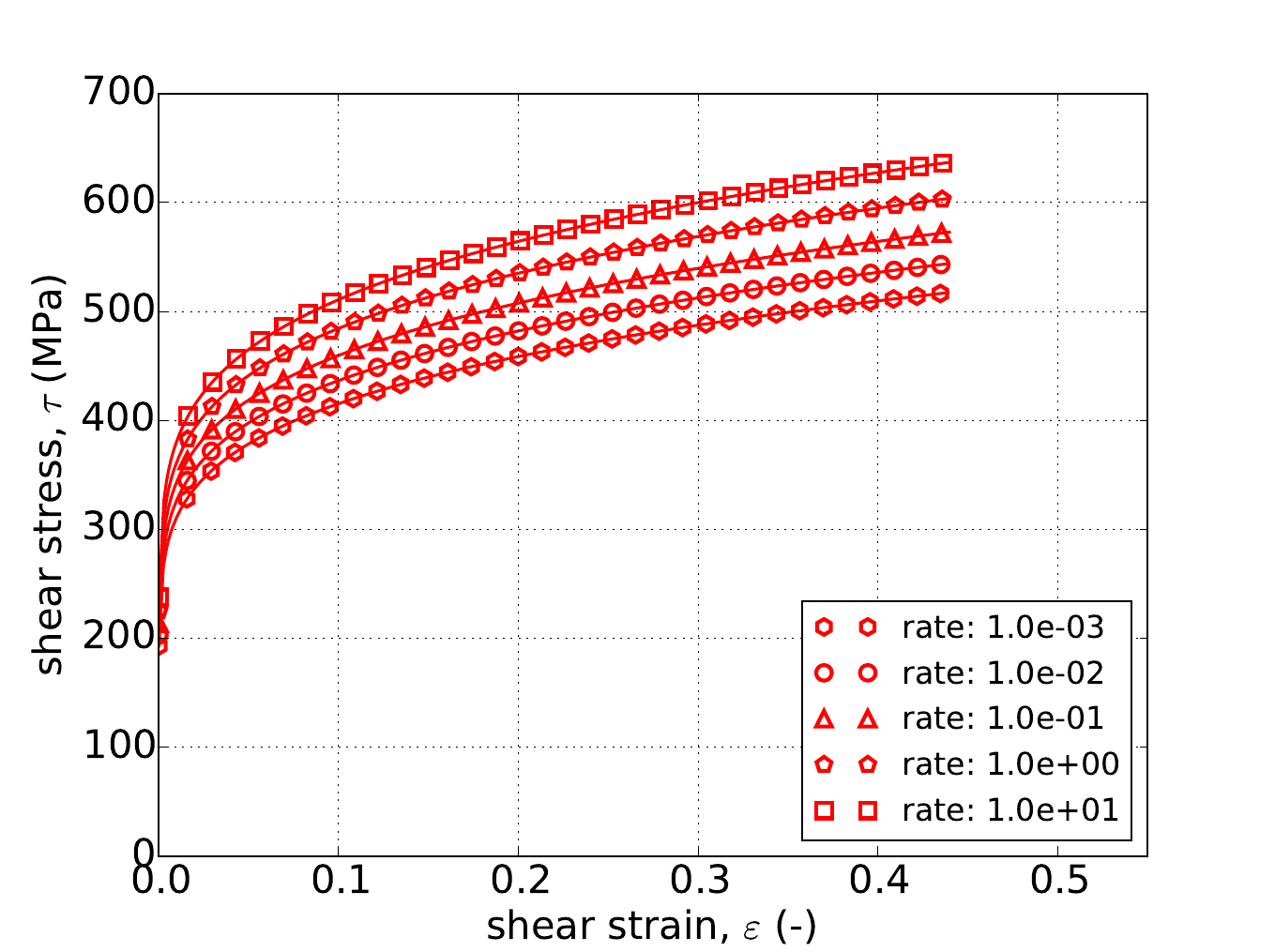
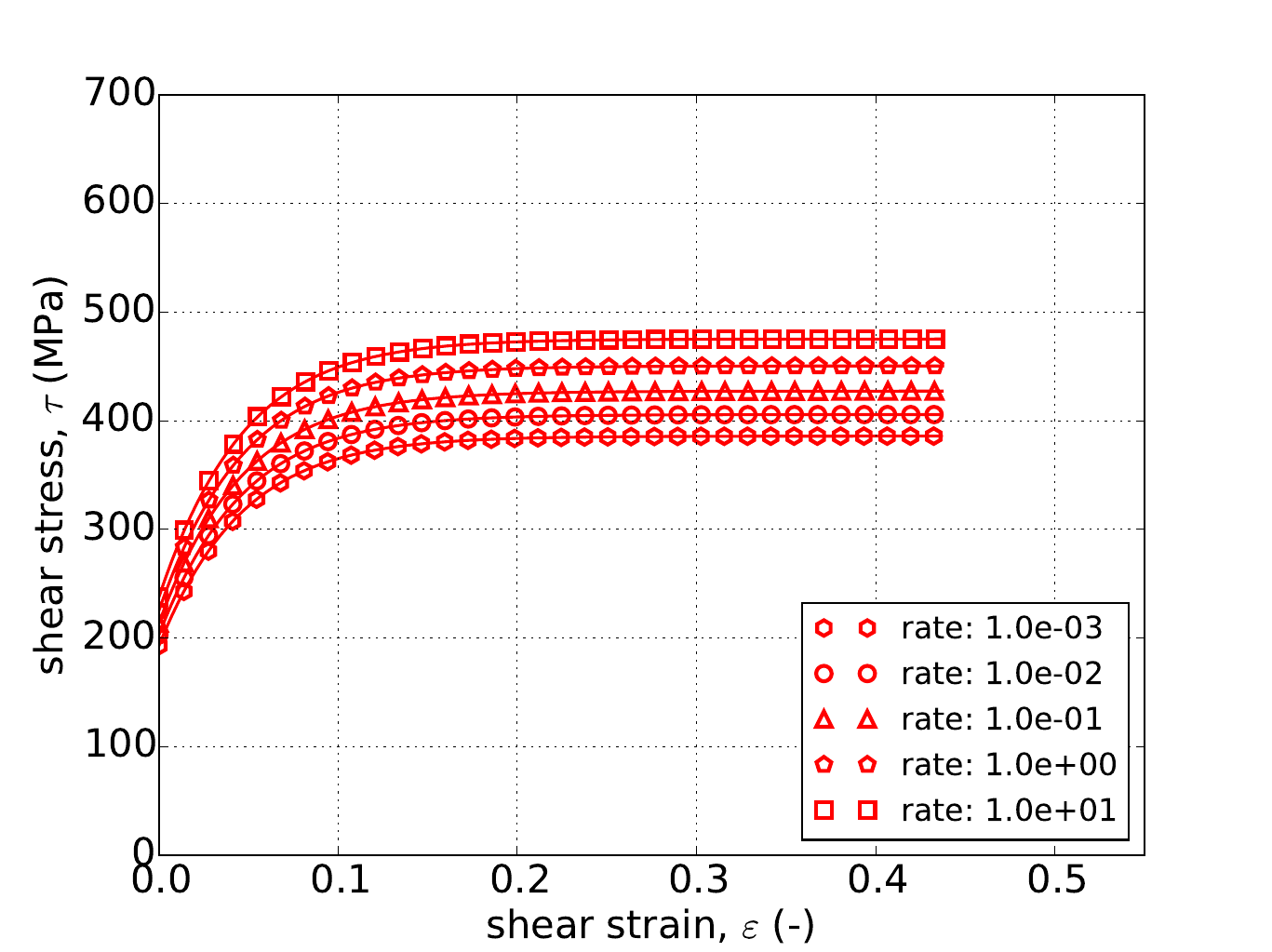
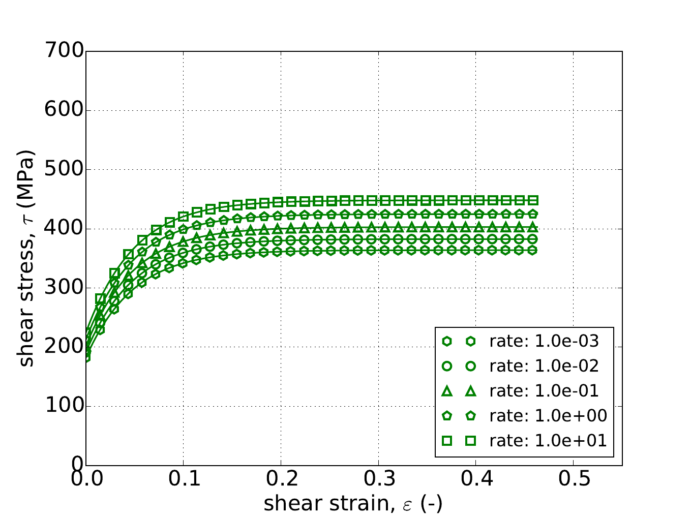
Similarly, Fig. 4.56 and Fig. 4.57 gives the results of the pure shear variant of the constant equivalent plastic strain rate verification test of Appendix A. The same five rates used in the uniaxial stress case are again utilized although in this instance as the pure shear response does depend on \(a\) the results are given for three yield surface exponents – \(a=~4,~8\) and \(20\). In the forty-five cases shown in Fig. 4.56 and Fig. 4.57 quite acceptable agreement is noted verifying the capabilities of the rate dependent Hosford implementation.

Linear Hardening, a=4

Linear Hardening, a=8

Linear Hardening, a=20

Power-Law Hardening, a=4

Power-Law Hardening, a=8

Power-Law Hardening, a=20

Fig. 4.56 Stress-strain response of the Hosford plasticity model with rate dependent, power-law breakdown type hardening in pure shear with (a-c) linear and (d-f) power-law rate independent hardening. Solid lines are analytical results while open symbols are numerical.

Power-Law Hardening, a=4

Power-Law Hardening, a=8

Power-Law Hardening, a=20

Fig. 4.57 Stress-strain response of the Hosford plasticity model with rate dependent, power-law breakdown type hardening in pure shear with (a-c) Voce rate independent hardening. Solid lines are analytical results while open symbols are numerical.

4.14.4. User Guide

BEGIN PARAMETERS FOR MODEL HOSFORD_PLASTICITY
  #
  # Elastic constants
  #
  YOUNGS MODULUS = <real>
  POISSONS RATIO = <real>
  SHEAR MODULUS  = <real>
  BULK MODULUS   = <real>
  LAMBDA         = <real>
  TWO MU         = <real>
  #
  # Yield surface parameters
  #
  YIELD STRESS = <real>
  A            = <real> (1.0)

#
  #
  # Hardening model
  #
  HARDENING MODEL = LINEAR | POWER_LAW | VOCE | USER_DEFINED |
  FLOW_STRESS | DECOUPLED_FLOW_STRESS | JOHNSON_COOK |
  POWER_LAW_BREAKDOWN
  #
  # Linear hardening
  #
  HARDENING MODULUS = <real>
  #
  # Power-law hardening
  #
  HARDENING CONSTANT = <real>
  HARDENING EXPONENT = <real> (0.5)
  LUDERS STRAIN      = <real> (0.0)
  #
  # Voce hardening
  #
  HARDENING MODULUS       = <real>
  EXPONENTIAL COEFFICIENT = <real>
  #
  # Johnson-Cook hardening
  #
  HARDENING FUNCTION = <string>hardening_function_name
  RATE CONSTANT      = <real>
  REFERENCE RATE     = <real>
  #
  # Power law breakdown hardening
  #
  HARDENING FUNCTION = <string>hardening_function_name
  RATE COEFFICIENT   = <real>
  RATE EXPONENT      = <real>
  # User defined hardening
  #
  HARDENING FUNCTION = <string>hardening_function_name
  #

#
  #
  # Following Commands Pertain to Flow_Stress Hardening Model
  #
  #    -  Isotropic Hardening model
  #
  ISOTROPIC HARDENING MODEL = LINEAR | POWER_LAW | VOCE |
                              USER_DEFINED
  #
  # Specifications for Linear, Power-law, and Voce same as above
  #
  # User defined hardening
  #
  ISOTROPIC HARDENING FUNCTION = <string>iso_hardening_fun_name
  #
  #     - Rate dependence
  #
  RATE MULTIPLIER = JOHNSON_COOK | POWER_LAW_BREAKDOWN |
     USER_DEFINED | RATE_INDEPENDENT (RATE_INDEPENDENT)
  #
  # Specifications for Johnson-Cook, Power-law-breakdown
  #     same as before EXCEPT no need to specify a
  #     hardening function
  #
  # User defined rate multiplier
  #
  RATE MULTIPLIER FUNCTION = <string> rate_mult_function_name
  #
  #     - Temperature dependence
  #
  TEMPERATURE MULTIPLIER = JOHNSON_COOK | USER_DEFINED |
     TEMPERATURE_INDEPENDENT (TEMPERATURE_INDEPENDENT)
  #
  #  Johnson-Cook temperature dependence
  #
  MELTING TEMPERATURE   = <real>
  REFERENCE TEMPERATURE = <real>
  TEMPERATURE EXPONENT  = <real>
  #
  #  User-defined temperature dependence
  TEMPERATURE MULTIPLIER FUNCTION = <string>temp_mult_function_name
  #
  # Following Commands Pertain to Decoupled_Flow_Stress Hardening Model
  #
  #    -  Isotropic Hardening model
  #
  ISOTROPIC HARDENING MODEL = LINEAR | POWER_LAW | VOCE | USER_DEFINED
  #
  # Specifications for Linear, Power-law, and Voce same as above
  #
  # User defined hardening
  #
  ISOTROPIC HARDENING FUNCTION = <string>isotropic_hardening_function_name
  #
  #     - Rate dependence
  #
  YIELD RATE MULTIPLIER = JOHNSON_COOK | POWER_LAW_BREAKDOWN |
              USER_DEFINED | RATE_INDEPENDENT (RATE_INDEPENDENT)
  #
  # Specifications for Johnson-Cook, Power-law-breakdown same as before
  #     EXCEPT no need to specify a hardening function
  #     AND should be preceded by YIELD
  #
  #     As an example for Johnson-Cook yield rate dependence,
  #
  YIELD RATE CONSTANT  = <real>
  YIELD REFERENCE RATE = <real>
  #
  # User defined rate multiplier
  #
  YIELD RATE MULTIPLIER FUNCTION = <string>yield_rate_mult_function_name
  #
  HARDENING_RATE MULTIPLIER = JOHNSON_COOK | POWER_LAW_BREAKDOWN |
              USER_DEFINED | RATE_INDEPENDENT (RATE_INDEPENDENT)
  #
  #     Syntax same as for yield parameters but with a HARDENING prefix
  #
  #     - Temperature dependence
  #
  YIELD TEMPERATURE MULTIPLIER = JOHNSON_COOK | USER_DEFINED |
            TEMPERATURE_INDEPENDENT (TEMPERATURE_INDEPENDENT)
  #
  #  Johnson-Cook temperature dependence
  #
  YIELD MELTING TEMPERATURE   = <real>
  YIELD REFERENCE TEMPERATURE = <real>
  YIELD TEMPERATURE EXPONENT  = <real>
  #
  #  User-defined temperature dependence
  YIELD TEMPERATURE MULTIPLIER FUNCTION = <string>yield_temp_mult_fun_name
  #
  HARDENING TEMPERATURE MULTIPLIER = JOHNSON_COOK | USER_DEFINED |
            TEMPERATURE_INDEPENDENT (TEMPERATURE_INDEPENDENT)
  #
  #   Syntax for hardening constants same as for yield but
  #            with HARDENING prefix

#
  #
  # Optional Failure Definitions
  #    Following only need to be defined if intend to use failure model
  #
  FAILURE MODEL = TEARING_PARAMETER | JOHNSON_COOK_FAILURE | WILKINS
                  | MODULAR_FAILURE | MODULAR_BCJ_FAILURE

  CRITICAL FAILURE PARAMETER = <real>
  #
  # TEARING_PARAMETER Failure model definitions
  #
  TEARING PARAMETER EXPONENT = <real>
  #
  # JOHNSON_COOK_FAILURE Failure model definitions
  #
  JOHNSON COOK D1       = <real>
  JOHNSON COOK D2       = <real>
  JOHNSON COOK D3       = <real>
  JOHNSON COOK D4       = <real>
  JOHNSON COOK D5       = <real>
  #
  #Following Johnson-Cook parameters can only be defined once.  As such, only
  #  needed if not previously defined via Johnson-Cook multipliers
  #  w/ flow-stress hardening.  Does need to be defined
  #  w/ Decoupled Flow Stress
  #
  REFERENCE RATE        = <real>
  REFERENCE TEMPERATURE = <real>
  MELTING TEMPERATURE   = <real>
  #
  # WILKINS Failure model definitions
  #
  WILKINS ALPHA    = <real>
  WILKINS BETA     = <real>
  WILKINS PRESSURE = <real>
  #
  #  MODULAR_FAILURE Failure model definitions
  #
  PRESSURE MULTIPLIER         = PRESSURE_INDEPENDENT | WILKINS
                                | USER_DEFINED (PRESSURE_INDEPENDENT)
  LODE ANGLE MULTIPLIER       = LODE_ANGLE_INDEPENDENT |
                                WILKINS (LODE_ANGLE_INDEPENDENT)
  TRIAXIALITY MULTIPLIER      = TRIAXIALITY_INDEPENDENT | JOHNSON_COOK
                                | USER_DEFINED (TRIAXIALITY_INDEPENDENT)
  RATE FAIL MULTIPLIER        = RATE_INDEPENDENT | JOHNSON_COOK
                                | USER_DEFINED (RATE_INDEPENDENT)
  TEMPERATURE FAIL MULTIPLIER = TEMPERATURE_INDEPENDENT | JOHNSON_COOK
                                | USER_DEFINED (TEMPERATURE_INDEPENDENT)
  #
  # Individual multiplier definitions
  #
  PRESSURE MULTIPLIER = WILKINS
  WILKINS ALPHA       = <real>
  WILKINS PRESSURE    = <real>
  #
  PRESSURE MULTIPLIER = USER_DEFINED
  PRESSURE MULTIPLIER FUNCTION = <string> pressure_multiplier_fun_name
  #
  LODE ANGLE MULTIPLIER = WILKINS
  WILKINS BETA          = <real>
  #
  TRIAXIALITY MULTIPLIER = JOHNSON_COOK
  JOHNSON COOK D1        = <real>
  JOHNSON COOK D2        = <real>
  JOHNSON COOK D3        = <real>
  #
  TRIAXIALITY MULTIPLIER = USER_DEFINED
  TRIAXIALITY MULTIPLIER FUNCTION = <string> triaxiality_multiplier_fun_name
  #
  RATE FAIL MULTIPLIER = JOHNSON_COOK
  JOHNSON COOK D4      = <real>
  # REFERENCE RATE should only be added if not previously defined
  REFERENCE RATE       = <real>
  #
  RATE FAIL MULTIPLIER = USER_DEFINED
  RATE FAIL MULTIPLIER FUNCTION = <string> rate_fail_multiplier_fun_name
  #
  TEMPERATURE FAIL MULTIPLIER = JOHNSON_COOK
  JOHNSON COOK D5             = <real>
  # JC Temperatures should only be defined if not previously given
  REFERENCE TEMPERATURE       = <real>
  MELTING TEMPERATURE         = <real>
  #
  TEMPERATURE FAIL MULTIPLIER          = USER_DEFINED
  TEMPERATURE FAIL MULTIPLIER FUNCTION = <string> temp_multiplier_fun_name
  #
  # MODULAR_BCJ_FAILURE Failure model definitions
  #
  INITIAL DAMAGE    = <real>
  INITIAL VOID SIZE = <real>
  DAMAGE BETA       = <real> (0.5)
  GROWTH MODEL      = COCKS_ASHBY | NO_GROWTH (NO_GROWTH)
  NUCLEATION MODEL  = HORSTEMEYER_GOKHALE | CHU_NEEDLEMAN_STRAIN
                      | NO_NUCLEATION (NO_NUCLEATION)
  #
  GROWTH RATE FAIL MULTIPLIER        = JOHNSON_COOK | USER_DEFINED
                                       | RATE_INDEPENDENT
                                       (RATE_INDEPENDENT)
  GROWTH TEMPERATURE FAIL MULTIPLIER = JOHNSON_COOK | USER_DEFINED
                                       | TEMPERATURE_INDEPENDENT
                                       (TEMPERATURE_INDEPENDENT)
  #
  NUCLEATION RATE FAIL MULTIPLIER        = JOHNSON_COOK | USER_DEFINED
                                           | RATE_INDEPENDENT
                                           (RATE_INDEPENDENT)
  NUCLEATION TEMPERATURE FAIL MULTIPLIER = JOHNSON_COOK | USER_DEFINED
                                           | TEMPERATURE_INDEPENDENT
                                           (TEMPERATURE_INDEPENDENT)
  #
  # Definitions for individual growth and nucleation models
  #
  GROWTH MODEL = COCKS_ASHBY
  DAMAGE EXPONENT = <real> (0.5)
  #
  NUCLEATION MODEL      = HORSTEMEYER_GOKHALE
  NUCLEATION PARAMETER1 = <real> (0.0)
  NUCLEATION PARAMETER2 = <real> (0.0)
  NUCLEATION PARAMETER3 = <real> (0.0)
  #
  NUCLEATION MODEL          = CHU_NEEDLEMAN_STRAIN
  NUCLEATION AMPLITUDE      = <real>
  MEAN NUCLEATION STRAIN    = <real>
  NUCLEATION STRAIN STD DEV = <real>
  #
  # Definitions for rate and temperature fail multiplier
  #   Note: only showing definitions for growth.
  #    Nucleation terms are the same just with NUCLEATION instead
  #    of GROWTH
  #
  GROWTH RATE FAIL MULTIPLIER = JOHNSON_COOK
  GROWTH JOHNSON COOK D4      = <real>
  GROWTH REFERENCE RATE       = <real>
  #
  GROWTH RATE FAIL MULTIPLIER          = USER_DEFINED
  GROWTH RATE FAIL MULTIPLIER FUNCTION = <string> growth_rate_fail_mult_func
  #
  GROWTH TEMPERATURE FAIL MULTIPLIER = JOHNSON_COOK
  GROWTH JOHNSON COOK D5             = <real>
  GROWTH REFERENCE TEMPERATURE       = <real>
  GROWTH MELTING TEMPERATURE         = <real>
  #
  GROWTH TEMPERATURE FAIL MULTIPLIER          = USER_DEFINED
  GROWTH TEMPERATURE FAIL MULTIPLIER FUNCTION = <string> temp_fail_mult_func
  #

#
  #
  # Optional Adiabatic Heating/Thermal Softening  Definitions
  #    Following only need to be defined if intend to use failure model
  #
  THERMAL SOFTENING MODEL = ADIABATIC | COUPLED
  #
  SPECIFIC HEAT = <real> # not needed for COUPLED
  BETA_TQ       = <real>

END [PARAMETERS FOR MODEL HOSFORD_PLASTICITY]

In the command blocks that define the Hosford plasticity model:

• The reference nominal yield stress, \(\bar{\sigma}\), is defined with the YIELD STRESS command line.

• The yield surface exponent, \(a\), is defined with the A command line.

• The type of hardening law is defined with the HARDENING MODEL command line, other hardening commands then define the specific shape of that hardening curve.

• The hardening modulus for a linear hardening model is defined with the HARDENING MODULUS command line.

• The hardening constant for a power law hardening model is defined with the HARDENING CONSTANT command line.

• The hardening exponent for a power law hardening model is defined with the HARDENING EXPONENT command line.

• The Luders strain for a power law hardening model is defined with the LUDERS STRAIN command line.

• The hardening function for a user defined hardening model is defined with the HARDENING FUNCTION command line.

• The shape of the spline for the spline based hardening is defined by the CUBIC SPLINE TYPE, CARDINAL PARAMETER, KNOT EQPS, and KNOT STRESS command lines.

Output variables available for this model are listed in Table 4.19.

Table 4.19 State Variables for HOSFORD PLASTICITY Model

Name	Description
EQPS	equivalent plastic strain, \(\bar{\varepsilon}^{p}\)
EQDOT	equivalent plastic strain rate, \(\dot{\bar{\varepsilon}}^{p}\)
SEFF	effective stress, \(\phi\)
TENSILE_EQPS	tensile equivalent plastic strain, \(\bar{\varepsilon}^{p}_{t}\)
DAMAGE	damage, \(\phi\)
VOID_COUNT	void count, \(\eta\)
VOID_SIZE	void size, \(\upsilon\)
DAMAGE_DOT	damage rate, \(\dot{\phi}\)
VOID_COUNT_DOT	void count rate, \(\dot{\eta}\)
PLASTIC_WORK_HEAT_RATE	plastic work heat rate, \(\dot{Q}^p\)

---

[1]

W.F. Hosford. A generalized isotropic yield criterion. Journal of Applied Mechanics, 39:607–609, 1972.

[2]

A. Graf and W. Hosford. Calculations of forming limit diagrams. Metallurgical Transactions A, 21A:87–94, 1990.

[3] (1,2,3,4)

W. M. Scherzinger. A return mapping algorithm for isotropic and anisotropic plasticity models using a line search method. Computer Methods in Applied Mechanics and Engineering, 317:526–553, 2017.

[4] (1,2)

B.T. Lester and W.M. Scherzinger. Failure formulations in modular plasticity models. Memo to distribution SAND2019-9678R, Sandia National Laboratories, Albuquerque, NM and Livermore, CA, 2019.

[5] (1,2)

B.T. Lester and W.M. Scherzinger. Modular growth and nucleation formulations in modular plasticity models. Memo to distribution SAND2020-7404R, Sandia National Laboratories, Albuquerque, NM and Livermore, CA, 2020.

[6] (1,2)

B.T. Lester and W.M. Scherzinger. Adiabatic heating in modular plasticity models. Memo to distribution SAND2019-15003R, Sandia National Laboratories, Albuquerque, NM and Livermore, CA, 2019.

[7]

R. Hill. The Mathematical Theory of Plasticity. Oxford University Press, 1950.

[8]

J. Lemaitre and J.-L. Chaboche. Mechanics of Solid Materials. Cambridge University Press, 1990.

[9]

J. Lubliner. Plasticity Theory. Dover, 2008.

[10]

G.R. Johnson and W.H. Cook. A constitutive model and data for metals subjected to large strains, high strain rates and high temperatures. In Proc. 7th. Int. Symp. on Ballistics, 541–547. The Hague, The Netherlands, 1983.

[11]

G.R. Johnson and W.H. Cook. Fracture characteristics of three metals subjected to various strains, strain rates, temperatures and pressures. Engineering Fracture Mechanics, 21(1):31–48, 1985.

[12]

H. J. Frost and M. F. Ashby. Deformation Mechanism Maps: the Plasticity and Creep of Metals and Ceramics. Pergamon Press, 1982.

[13]

A.A. Brown and D.J. Bammann. Validation of a model for static and dynamic recrystallization in metals. International Journal of Plasticity, 32–33:17–35, 2012.

[14]

F. Armero and A. Pèrez-Foguet. On the formulation of closes-point projection algorithms in elastoplasticity – part I: The variational structure. International Journal for Numerical Methods in Engineering, 53:297–329, 2002.

[15]

A. Pèrez-Foguet and F. Armero. On the formulation of closest-point projection algorithms in elastoplasticity – part II: Globally convergent schemes. International Journal for Numerical Methods in Engineering, 53:331–374, 2002.

[16]

F. Barlat, H. Aretz, J. W. Yoon, J. C. Brem, and R. E. Dick. Linear transformation-based anisotropic yield functions. International Journal of Plasticity, 21:1009–1039, 2005.