4.21. Munson-Dawson Viscoplastic Model

4.21.1. Theory

The Munson-Dawson (MD) model was originally defined in [[1], [2], [3]], but several changes were made in [[4]]. This section presents the current model in a small strain setting. (Section 4.21.2 briefly mentions how the model is extended into the finite deformation realm.) Note that compressive stresses and strains are treated as positive in this section, as is common in the geomechanics literature.

The MD model is an isotropic, hypoelastic, unified viscoplastic, material model. The total strain rate \(\dot{\varepsilon}_{ij}\) is decomposed into an elastic strain rate \(\dot{\varepsilon}^\mathrm{el}_{ij}\), a thermal strain rate \(\dot{\varepsilon}^\mathrm{th}_{ij}\), and a viscoplastic strain rate \(\dot{\varepsilon}^\mathrm{vp}_{ij}\):

(4.89)\[\dot{\varepsilon}_{ij} = \dot{\varepsilon}^\mathrm{el}_{ij} + \dot{\varepsilon}^\mathrm{th}_{ij} + \dot{\varepsilon}^\mathrm{vp}_{ij}.\]

The elastic portion of the MD model utilizes the following simple linear relationship between \(\dot{\varepsilon}^\mathrm{el}_{kl}\) and the stress rate \(\dot{\sigma}_{ij}\),

(4.90)\[\dot{\sigma}_{ij} = \mathbb{C}_{ijkl}\dot{\varepsilon}^\mathrm{el}_{kl} = \mathbb{C}_{ijkl}\left(\dot{\varepsilon}_{kl} - \dot{\varepsilon}^\mathrm{th}_{kl} - \dot{\varepsilon}^\mathrm{vp}_{kl}\right)\]

(4.91)\[\mathbb{C}_{ijkl} = (B-2/3\,\mu)\,\delta_{ij}\,\delta_{kl} + \mu\,\left(\delta_{ik}\,\delta_{jl} + \delta_{il}\,\delta_{jk}\right) ,\]

where \(\mathbb{C}_{ijkl}\) is the elastic stiffness, which is composed of the bulk modulus \(B\), the shear modulus \(\mu\), and the Kronecker Delta \(\delta_{ij}\). The thermal strain portion of the model is simply

(4.92)\[\dot{\varepsilon}^\mathrm{th}_{ij} = -\alpha\,\dot{\theta}\,\delta_{ij}\]

where \(\alpha\) is the coefficient of thermal expansion, and \(\theta\) is the temperature. Sierra/SM also offers thermal strain functions for adding thermal strain effects to any given model. If \(\alpha\ne0\), then MD model users should not specify a thermal strain function, otherwise thermal strains will be applied twice.

Plastic deformation is assumed to be isochoric and only occurs in the presence of shear stress. The MD model utilizes the Hosford stress as its equivalent shear stress measure \(\bar{\sigma}\). The Hosford stress is

(4.93)\[\bar{\sigma} = \left\{\frac{1}{2}\left[|\sigma_1 - \sigma_2|^a + |\sigma_2 - \sigma_3|^a + |\sigma_1 - \sigma_3|^a\right]\right\}^{1/a},\]

where \(\sigma_i\) are the principal stresses and \(a\) is a material parameter. This definition for \(\bar{\sigma}\) was proposed in [[5]] because it encompasses the Tresca stress (\(a=1\)), the von Mises stress (\(a=2\)), and a range of behaviors in-between (\(1<a<2\)). One can also reproduce the Tresca stress with \(a=\infty\), the von Mises stress with \(a=4\), and behaviors in-between with \(4<a<\infty\). This second range avoids potential singularities in the first and second derivatives of (4.93), so the exponent is restricted to \(a\ge4\).

The viscoplastic strain evolves according to an associated flow rule

(4.94)\[\dot{\varepsilon}^\mathrm{vp}_{ij} = \dot{\bar{\varepsilon}}^\mathrm{vp}\frac{\partial\bar{\sigma}}{\partial\sigma_{ij}},\]

where \(\dot{\bar{\varepsilon}}^\mathrm{vp}\) is the equivalent viscoplastic strain rate. It can be decomposed into two components

(4.95)\[\dot{\bar{\varepsilon}}^\mathrm{vp} = \dot{\bar{\varepsilon}}^\mathrm{tr} + \dot{\bar{\varepsilon}}^\text{ss},\]

where \(\dot{\bar{\varepsilon}}^\mathrm{tr}\) is the transient equivalent viscoplastic strain rate and \(\dot{\bar{\varepsilon}}^\text{ss}\) is the steady state equivalent viscoplastic strain rate.

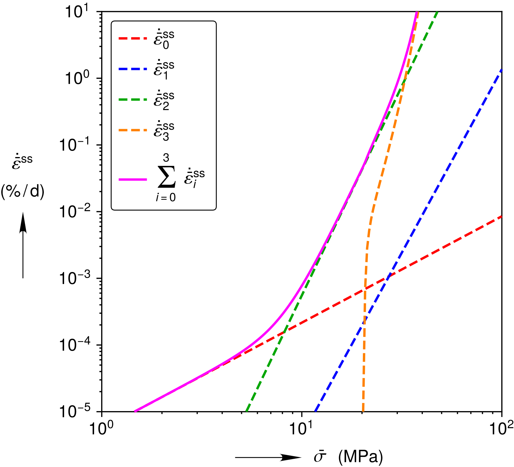
The MD model decomposes the steady state behavior into four mechanisms:

(4.96)\[\begin{split}\dot{\bar{\varepsilon}}^\text{ss} =& \sum^3_{i=0} \dot{\bar{\varepsilon}}^\text{ss}_i \notag \\ \dot{\bar{\varepsilon}}^\text{ss}_i =& A_i\,\exp\left(-\frac{Q_i}{R\,\theta}\right)\,\left(\frac{\bar{\sigma}}{\mu}\right)^{n_i} \quad \text{for } i=0, 1, \text{ and } 2 \\ \dot{\bar{\varepsilon}}^\text{ss}_3 =& H(\bar{\sigma}-\bar{\sigma}_{\text{g}})\sum^2_{i=0}B_i\,\exp\left(-\frac{Q_i}{R\,\theta}\right)\,\mathrm{sinh}\left(q\frac{(\bar{\sigma}-\bar{\sigma}_{\text{g}})}{\mu}\right),\end{split}\]

The variables \(A_i\), \(B_i\), \(Q_i\), \(n_i\), \(\bar{\sigma}_{\text{g}}\), and \(q\) are all model parameters. All four mechanisms have an Arrhenius temperature dependence, where \(Q_i\) is an activation energy and \(R=8.314\)J/(K mol) is the universal gas constant. Mechanism 3 is only activated when \(\bar{\sigma}\) exceeds \(\bar{\sigma}_{\text{g}}\), as reflected in the heaviside function \(H(\bar{\sigma}-\bar{\sigma}_{\text{g}})\). Typically, the parameters \(B_i\) are chosen to produce a smooth transition to mechanism 3 at \(\bar{\sigma}_{\text{g}}\).

The simple functional forms of (4.96) suffice for the steady-state behavior, but the transient behavior is somewhat more complex. During work hardening under constant stress, \(\dot{\bar{\varepsilon}}^\mathrm{tr}\) approaches the transient strain limit \(\dot{\bar{\varepsilon}}^\mathrm{tr*}\) from below, and the total viscoplastic strain rate slows down over time. During recovery under constant stress, \(\dot{\bar{\varepsilon}}^\mathrm{tr}\) approaches \(\dot{\bar{\varepsilon}}^\mathrm{tr*}\) from above, and the total viscoplastic strain rate speeds up over time. The rate that \(\dot{\bar{\varepsilon}}^\mathrm{tr}\) approaches \(\dot{\bar{\varepsilon}}^\mathrm{tr*}\) is governed by

(4.97)\[\dot{\bar{\varepsilon}}^\mathrm{tr} = \left(F-1\right)\,\dot{\bar{\varepsilon}}^\text{ss},\]

where

(4.98)\[F = \exp\left[\mathrm{\mathrm{sign}\,}\,(\dot{\bar{\varepsilon}}^\mathrm{tr*} - \dot{\bar{\varepsilon}}^\mathrm{tr})\,\kappa\,\left(1-\displaystyle{\frac{\dot{\bar{\varepsilon}}^\mathrm{tr}}{\dot{\bar{\varepsilon}}^\mathrm{tr*}}}\right)^2\right].\]

and \(\kappa\) is a quantity that depends on whether the material is work hardening or recovering. These two behaviors are captured in the following equations

(4.99)\[\begin{split}\kappa = \begin{cases} \alpha_{\mathrm{h}} + \beta_{\text{h}}\,\log_{10}\left(\displaystyle{\frac{\bar{\sigma}}{\mu}}\right) & \dot{\bar{\varepsilon}}^\mathrm{tr} \leq \dot{\bar{\varepsilon}}^\mathrm{tr*} \\ \alpha_{\mathrm{r}} + \beta_{\text{r}}\,\log_{10}\left(\displaystyle{\frac{\bar{\sigma}}{\mu}}\right) & \dot{\bar{\varepsilon}}^\mathrm{tr} > \dot{\bar{\varepsilon}}^\mathrm{tr*}. \end{cases}\end{split}\]

where \(\alpha_j\) and \(\beta_j\) are model parameters. Note that the parameter \(\kappa\) must be non-negative, otherwise (4.97) produces a negative/positive \(\dot{\bar{\varepsilon}}^\mathrm{tr}\) when \(\dot{\bar{\varepsilon}}^\mathrm{tr}\) is below/above \(\dot{\bar{\varepsilon}}^\mathrm{tr*}\). (Such behavior occurs during reverse creep, but the MD model is only designed to model forward creep.) To enforce this, (4.99) is calculated first, and then

\[\kappa \leftarrow \max(\kappa, 0)\]

is applied.

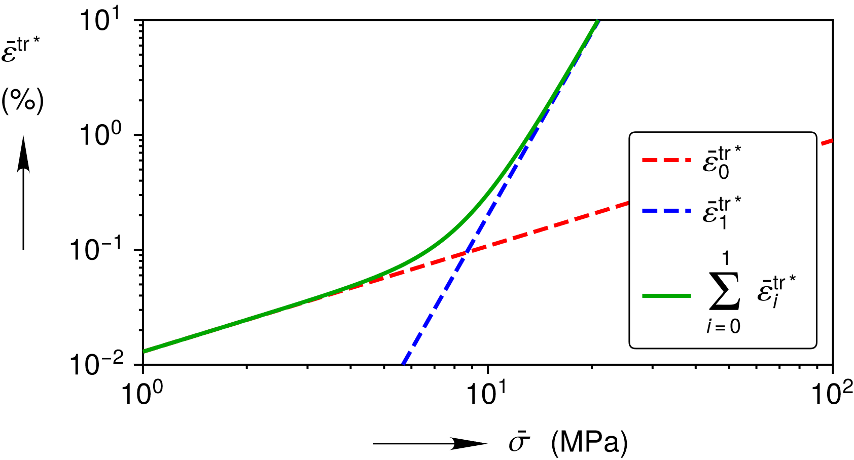
The MD model uses two mechanisms to endow \(\dot{\bar{\varepsilon}}^\mathrm{tr*}\) with stress and temperature dependence:

(4.100)\[\begin{split}\dot{\bar{\varepsilon}}^\mathrm{tr*} &= \sum^1_{i=0} \dot{\bar{\varepsilon}}^\mathrm{tr*}_i \notag \\ \dot{\bar{\varepsilon}}^\mathrm{tr*}_i &= K_i\,\exp(c_i\,\theta)\left(\frac{\bar{\sigma}}{\mu}\right)^{m_i},\end{split}\]

where \(K_i\), \(c_i\), and \(m_i\) are parameters to be calibrated against experimental results.

4.21.2. Implementation

The full details of the MD model’s numerical implementation are published in [[4]]. This section discusses several salient points for the typical MD model user and to define all the input parameters in Section 4.21.4.

• As discussed in Section 4.21.3, one can obtain an analytical solution to the MD model’s ordinary differential equations if the exponent in (4.98) is changed from 2 to 1, and \(\mathrm{\mathrm{sign}\,}\,(\dot{\bar{\varepsilon}}^\mathrm{tr*} - \dot{\bar{\varepsilon}}^\mathrm{tr})=1\). To accommodate this possibility, (4.98) is numerically implemented as

(4.101)\[F = \exp\left[\mathrm{\mathrm{sign}\,}\,(\dot{\bar{\varepsilon}}^\mathrm{tr*} - \dot{\bar{\varepsilon}}^\mathrm{tr})^{\chi-1}\,\kappa\,\left(1-\displaystyle{\frac{\dot{\bar{\varepsilon}}^\mathrm{tr}}{\dot{\bar{\varepsilon}}^\mathrm{tr*}}}\right)^\chi\right]\]

where \(\chi\) is a user specified integer that is equal to 2 by default, but one can set \(\chi = 1\) for verification testing.

• Each steady state creep mechanism is implemented with a viscoplastic rate scale factor \(s\), such that (4.96) becomes

(4.102)\[\begin{split}\dot{\bar{\varepsilon}}^\text{ss} =& \sum^3_{i=0} \dot{\bar{\varepsilon}}^\text{ss}_i \notag \\ \dot{\bar{\varepsilon}}^\text{ss}_i =& s\,A_i\,\exp\left(-\frac{Q_i}{R\,\theta}\right)\,\left(\frac{\bar{\sigma}}{\mu}\right)^{n_i} \quad \text{for} i=0, 1, and 2 \\ \dot{\bar{\varepsilon}}^\text{ss}_3 =& s\,H(\bar{\sigma}-\bar{\sigma}_{\text{g}})\,\sum^2_{i=0}B_i\,\exp\left(-\frac{Q_i}{R\,\theta}\right)\,\mathrm{sinh}\left(q\frac{(\bar{\sigma}-\bar{\sigma}_{\text{g}})}{\mu}\right).\end{split}\]

This scale factor can be used to speed up or slow down the equivalent steady-state strain rate and the total equivalent viscoplastic strain rate, because \(\dot{\bar{\varepsilon}}^\mathrm{vp}=\dot{\bar{\varepsilon}}^\mathrm{tr} + \dot{\bar{\varepsilon}}^\text{ss} = F\,\dot{\bar{\varepsilon}}^\text{ss}\). The default value is \(s=1\), but it can be useful to set \(s\) to some small value to “freeze” the material’s viscoplasticity for a period of time, or increase \(s\) to larger values to squeeze hundreds of years into a few seconds. Speeding up the viscoplasticity can allow one to make quasi-static simulations using explicit dynamics, provided inertial effects are kept to a minimum. The variable \(s\) is implemented as an internal state variable, rather than a material parameter, so a user can modify it in the middle of a simulation. Internal state variables can be altered by creating a user variable with the same name as the internal state variable (viscoplastic_rate_scale_factor in this case) in a Sierra input deck and modifying the user variable with a user function or user subroutine (see Sections 2.3 and A.2.1 in [[6]]).

• The MD model is extended into the finite-deformation realm using hypoelasticity. Consistent with the Green-McInnis stress rate, the infinitesimal strain rates are replaced with the corresponding unrotated rates of deformation (i.e. \(\dot{\varepsilon}_{ij}\rightarrow D_{ij}\)) and the stress is replaced with the unrotated Cauchy stress (\(\sigma_{ij}\rightarrow T{ij}\)).

• Following the lead of Scherzinger [[7]], the model’s time derivatives are discretized using the backwards Euler method, and the resulting non-linear algebraic equations are solved with a line search augmented Newton-Raphson method.

A typical user of the model should not need to adjust the routine’s default numerical parameters, but the parameters are briefly mentioned here should adjustment become necessary.

• The implementation has some expressions where \(\bar{\sigma}\) is in the denominator of a fraction. If an initial calculation of the Hosford stress results in \(\bar{\sigma}<\bar{\sigma}_{\text{min}}\), then the initial value is replaced with \(\bar{\sigma}_{\text{min}}\). The value of \(\bar{\sigma}_{\text{min}}\) should be small enough to have negligible impact, yet still avoid \(\bar{\sigma}=0\).

• Each iteration of the implicit integration routine updates the merit function \(\omega^{(k)}=1/2\left(\mathcal{R}^{(k)}_{ij}\mathcal{R}^{(k)}_{ij} + {r^{(k)}}^2\right)\) for iteration \(k\), where \(\mathcal{R}^{(k)}_{ij}\) and \(r^{(k)}\) are the residuals associated with the differential equations in (4.94) and (4.97), respectively. An iteration is considered converged when \(\sqrt{\omega^{(k)}}<\sqrt{\omega_{\text{max}}}\). The value of \(\sqrt{\omega_{\text{max}}}\) should be a small positive value close to zero.

• If a Newton iteration (or a line search iteration) does not produce sufficient decrease in \(\omega^{(k)}\), a line search iteration is performed. The line search algorithm selects \(\zeta^{(j)}\), for each iteration \(j\), to search for a sufficient decrease in \(\omega^{(k)}(\zeta^{(j)})\) along the search direction provided by the Newton iteration. The start and end of the last Newton iteration are \(\zeta^{(j)}=0\) and \(\zeta^{(j)}=1\), respectively. A decrease in \(\omega^{(k)}(\zeta^{(j)})\) is considered sufficient if \(\omega^{(k)}(\zeta^{(j)}) < (1-2\,\xi\,\zeta^{(j-1)})\,\omega^{(k)}(0)\), where \(\xi\) is a positive value usually set close to zero.

• The minimum allowed value of \(\zeta^{(j)}\) is \(\gamma\).

• The maximum number of Newton iterations is \(k_{\text{max}}\).

• The maximum number of line search iterations is \(j_{\text{max}}\).

See [[4]] for further discussion of these numerical parameters.

4.21.3. Verification

The MD model contains ordinary differential equations ((4.94) and (4.97)) that make it non-trivial to verify. A straightforward analytical solution, however, can be constructed to these equations if \(\chi=1\) in (4.101) and if the stresses and temperatures remain piecewise constant in time.

Temporally constant stresses and temperatures allow (4.90), (4.91), (4.92), (4.93), (4.94), (4.95), and (4.96) to be integrated to

(4.103)\[\varepsilon_{kl} - \varepsilon_{kl}(t_j) = \mathbb{C}_{klmn}^{-1}\left(\sigma_{mn} - \sigma_{mn}(t_j)\right) - \alpha\,\left(\theta - \theta(t_j)\right)\,\delta_{kl} + \varepsilon^\mathrm{vp}_{kl} - \varepsilon^\mathrm{vp}_{kl}(t_j)\]

(4.104)\[\varepsilon^\mathrm{vp}_{kl} - \varepsilon^\mathrm{vp}_{kl}(t_j) = \left[\dot{\bar{\varepsilon}}^\mathrm{tr} - \dot{\bar{\varepsilon}}^\mathrm{tr}(t_j) + \dot{\bar{\varepsilon}}^\text{ss}\,(t-t_j)\right]\,\frac{\partial\bar{\sigma}}{\partial\sigma_{kl}}\]

where \(t_j\) is the time at the end of the previous time period \(j\). The quantities from the previous time period (\(\varepsilon_{kl}(t_j)\), \(\sigma_{mn}(t_j)\), \(\theta(t_j)\), \(\varepsilon^\mathrm{vp}_{kl}(t_j)\), and \(\dot{\bar{\varepsilon}}^\mathrm{tr}(t_j)\)) are assumed to be known. Setting \(\chi=1\) in (4.101) enables the following general analytical solution to (4.97):

(4.105)\[\dot{\bar{\varepsilon}}^\mathrm{tr} = \frac{\dot{\bar{\varepsilon}}^\mathrm{tr*}}{\kappa}\,\ln\left\{\exp(\kappa) + \exp\left[\frac{\kappa}{\dot{\bar{\varepsilon}}^\mathrm{tr*}} \, (C_1 - \dot{\bar{\varepsilon}}^\text{ss} t)\right]\right\}.\]

One can solve for the integration constant \(C_1\) using the initial condition \(\dot{\bar{\varepsilon}}^\mathrm{tr} = \dot{\bar{\varepsilon}}^\mathrm{tr}(t_j)\) at \(t=t_j\). After substituting the result back into (4.105), one obtains

(4.106)\[\dot{\bar{\varepsilon}}^\mathrm{tr} = \frac{\dot{\bar{\varepsilon}}^\mathrm{tr*}}{\kappa}\,\ln\left\{\exp(\kappa) + \left[\exp\left(\frac{\dot{\bar{\varepsilon}}^\mathrm{tr}(t_j)\,\kappa}{\dot{\bar{\varepsilon}}^\mathrm{tr*}}\right) - \exp(\kappa)\right]\,\exp\left[-\frac{\kappa}{\dot{\bar{\varepsilon}}^\mathrm{tr*}} \, \dot{\bar{\varepsilon}}^\text{ss} \, (t - t_j)\right]\right\}.\]

Combining (4.103), (4.104), and (4.106) produces the following closed form expression for the total strain change over a time period

(4.107)\[\begin{split}\varepsilon_{kl} - \varepsilon_{kl}(t_j) &= \mathbb{C}_{klmn}^{-1}\left(\sigma_{mn} - \sigma_{mn}(t_j)\right) - \alpha\,\left(\theta - \theta(t_j)\right)\,\delta_{kl} + \nonumber \\ & \Bigg[\frac{\dot{\bar{\varepsilon}}^\mathrm{tr*}}{\kappa}\,\ln\left\{\exp(\kappa) + \left[\exp\left(\frac{\dot{\bar{\varepsilon}}^\mathrm{tr}(t_j)\,\kappa}{\dot{\bar{\varepsilon}}^\mathrm{tr*}}\right) - \exp(\kappa)\right]\, \exp\left[-\frac{\kappa}{\dot{\bar{\varepsilon}}^\mathrm{tr*}} \, \dot{\bar{\varepsilon}}^\text{ss} \, (t - t_j)\right]\right\} \nonumber \\ &- \dot{\bar{\varepsilon}}^\mathrm{tr}(t_j) + \dot{\bar{\varepsilon}}^\text{ss}\,(t-t_j)\Bigg]\,\frac{\partial\bar{\sigma}}{\partial\sigma_{kl}}.\end{split}\]

The next three subsections compare numerical solutions against analytical solutions for axisymmetric compression, pure shear, and unequal biaxial compression. In each case, the numerical solution for the total strain is denoted as \(\varepsilon_{ij}\), while the analytical solution for the total strain in (4.107) is denoted as \(\hat{\varepsilon}_{ij}\). All the verification tests only involve principal deformations, so hypoelasticity simply reinterprets the stress and strain in Section 4.21.1 as the Cauchy stress and logarithmic strain, respectively. As a reminder, compressive stresses and strains are treated as positive.

All the verification tests utilize Calibration 3B of the MD model. The full parameter set can be found in [[4]], but Fig. 4.99, Fig. 4.100 and Fig. 4.101 depict much of the calibration graphically. Fig. 4.99 shows the shape of the Hosford equivalent stress surface for \(a=16\). The Hosford surface and the angle \(\phi\) of its normal \(n_{ij}\) depend on the Lode angle \(\phi\) of the deviatoric stress \(\sigma^{\text{dev}}_{ij}=\sigma_{ij}-1/3\sigma_{kk}\,\delta_{ij}\). Fig. 4.100 and Fig. 4.101 show the individual mechanisms \(\dot{\bar{\varepsilon}}^\mathrm{tr*}_i\) and \(\dot{\bar{\varepsilon}}^\text{ss}_i\), as well as the sums \(\dot{\bar{\varepsilon}}^\mathrm{tr*}=\sum_{i=0}^1 \dot{\bar{\varepsilon}}^\mathrm{tr*}_i\) and \(\dot{\bar{\varepsilon}}^\text{ss}=\sum_{i=0}^3 \dot{\bar{\varepsilon}}^\text{ss}_i\), so that one can visualize where each mechanism dominates the total behavior.

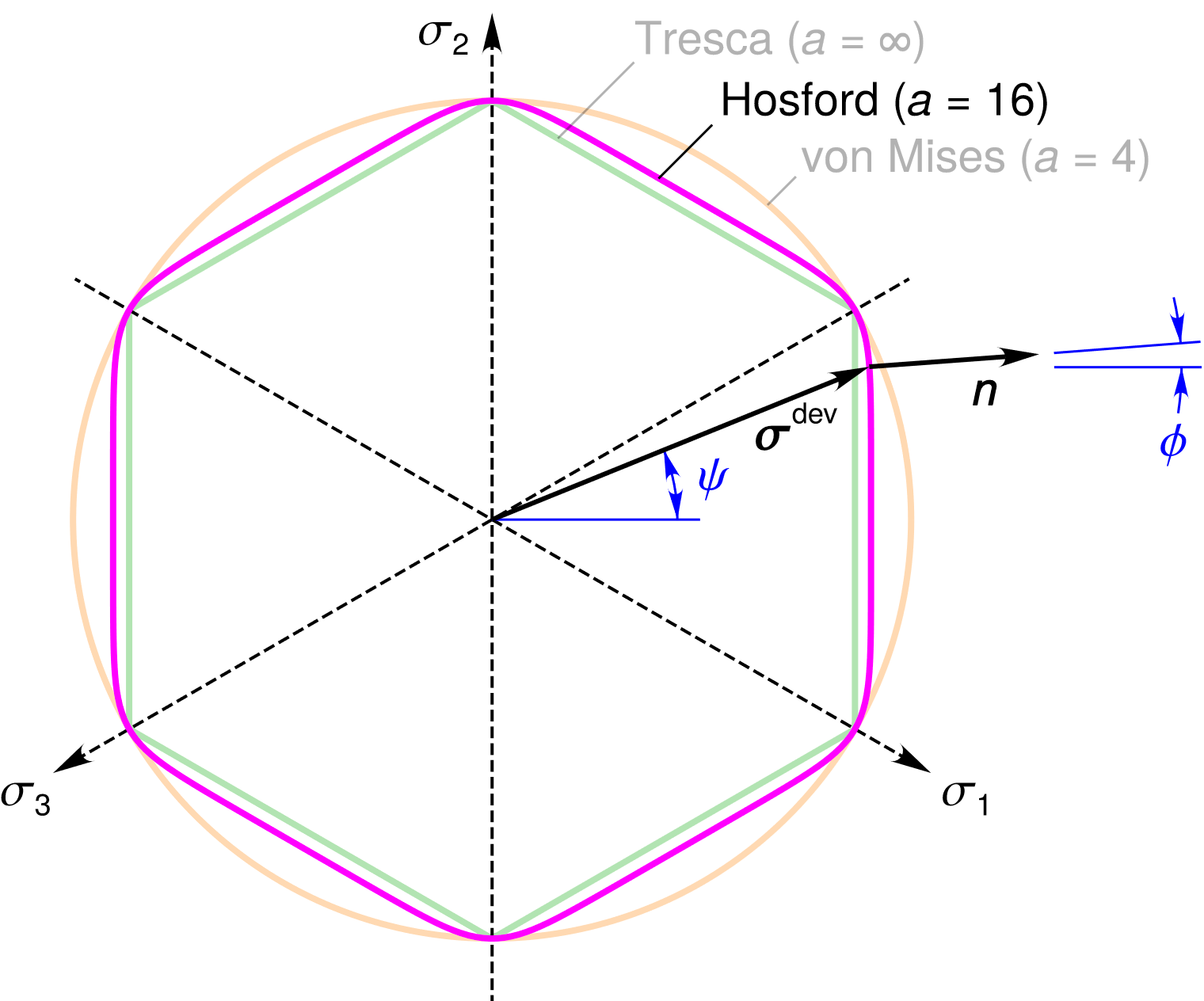
Fig. 4.99 Hosford equivalent stress surface in the \(\pi\)-plane.

Stress Dependence at 27 C

Temperature Dependence at 8 MPa

Fig. 4.100 Stress and temperature dependence of the transient strain limit for Calibration 3B.

Stress Dependence at 27 C

Temperature Dependence at 8 MPa

Fig. 4.101 Stress and temperature dependence of the steady-state strain rate for Calibration 3B.

4.21.3.1. Triaxial Compression

Triaxial compression tests are frequently used to characterize the creep and strength behavior of geomaterials, such as rock salt. Cylindrical specimens are subjected to a radial confining pressure \(\sigma_{\text{rr}}\) and an axial stress \(\sigma_{\text{zz}}\). Axisymmetric compression is perhaps a more appropriate name for these tests, because the hoop stress \(\sigma_{\vartheta\vartheta}\) is equal to \(\sigma_{\text{rr}}\), but triaxial compression is the common name.

Fig. 4.102 Triaxial Compression Verification Test

The applied stress and temperature histories for the test are shown in the top two plots in Fig. 4.102. The test begins with an isothermal, 20~MPa hydrostatic, hold period for 10 days, where the strain is purely elastic. At \(t=0\), \(\sigma_{\text{zz}}\) is increased to 35~MPa, while the other stresses are held fixed, causing a 15~MPa equivalent stress. This stress state is held for the next 50 days. The strain evolves quickly at first, but slows down to the steady-state rate as the material work hardens. At \(t=50\), \(\sigma_{\text{zz}}\) is decreased to 33~MPa, while the other stresses are held fixed. The 2~MPa drop in \(\bar{\sigma}\) causes the strain rate to slow down markedly, but it gradually builds to a new steady-state rate as the material recovers over the next 50 days.

In summary, the numerical and analytical solutions for the total strain match very well throughout the test, which verifies:

• Linear elasticity under triaxial compression

• Zero viscoplastic strain evolution under hydrostatic loading

• Viscoplastic strain evolution for \(\psi=-30^\circ\)

• Work hardening (\(\dot{\bar{\varepsilon}}^\mathrm{tr}<\dot{\bar{\varepsilon}}^\mathrm{tr*}\)) dominated by transient strain limit mechanism 1

• Recovery (\(\dot{\bar{\varepsilon}}^\mathrm{tr}>\dot{\bar{\varepsilon}}^\mathrm{tr*}\)) dominated by transient strain limit mechanism 1

• Steady-state strain accumulation dominated by transient strain limit mechanism 2.

4.21.3.2. Pure Shear

The Hosford equivalent stress depends on \(a\) for \(-30\deg<\psi<30\deg\), but it is independent of \(a\) for \(\psi=-30^\circ\) (triaxial compression) and \(\psi=30^\circ\) (triaxial extension). Pure shear is a simple stress state that exercises the Hosford stress at a Lode angle other than \(\psi=\pm30^\circ\). Pure shear can be expressed in the principal frame as \(\sigma_3=-\sigma_1\) and \(\sigma_2=0\). In addition to exercising the model under pure shear, this test also varies the temperature to verify thermal expansion and creep at elevated temperatures.

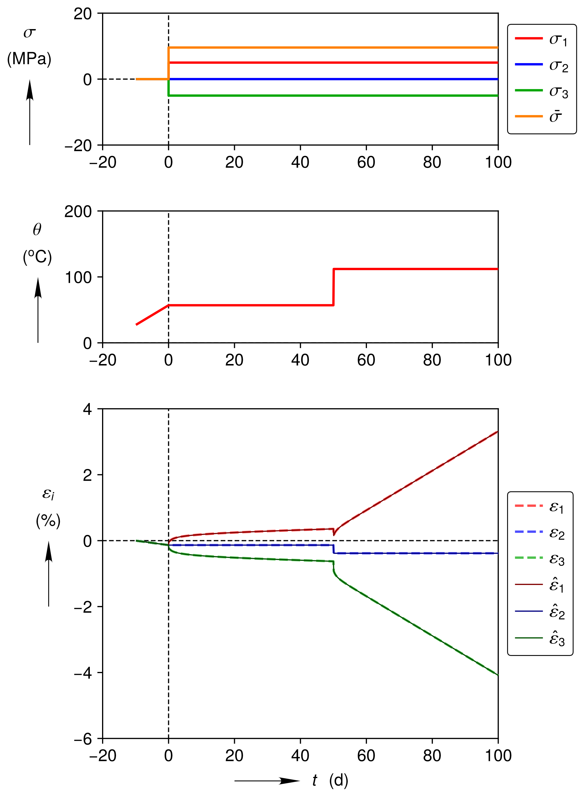
Fig. 4.103 Pure Shear Verification Test

The applied stress and temperature histories for the test are shown in the top two plots in Fig. 4.103. The test begins with a 0~MPa hydrostatic hold period for 10 days while the temperature is linearly ramped from 27\({}^\circ\)C to 57\({}^\circ\)C. Some thermal strains develop during this time. At \(t=0\) , the temperature ramp stops, \(\sigma_{\text{1}}\) is increased to 5~MPa, \(\sigma_{\text{2}}\) is held at zero, and \(\sigma_{\text{3}}\) is reduced to -5~MPa. This state is held for the next 50 days, while the material creeps. At \(t=50\), \(\theta\) is increased to 112\({}^\circ\)C, but the stresses remain fixed. The sharp increase in \(\theta\) causes a step change in thermal strain, and then accelerated creep is observed over the over the next 50 days.

In summary, the numerical and analytical solutions for the total strain match very well throughout the test, which verifies:

• Linear elasticity under pure shear

• Thermal expansion

• Viscoplastic strain evolution for \(\psi=0^\circ\)

• Temperature dependence of transient strain limit mechanism 1

• Steady-state strain accumulation dominated by mechanism 1

• Steady-state strain accumulation dominated by mechanism 2.

4.21.3.3. Unequal Biaxial Compression

Unequal biaxial compression is another stress state that exercises the Hosford stress at a Lode angle other than \(\psi=\pm30^\circ\). Unequal compressive stresses \(\sigma_{\text{xx}}\) and \(\sigma_{\text{yy}}\) are applied to two faces of a cube, while \(\sigma_{\text{zz}} = 0\). This stress state is slightly more complex than triaxial compression or pure shear because all three stress magnitudes are unequal. This test also alters the stress component ratios after 50 days of creep to verify the model’s ability to change Lode angle.

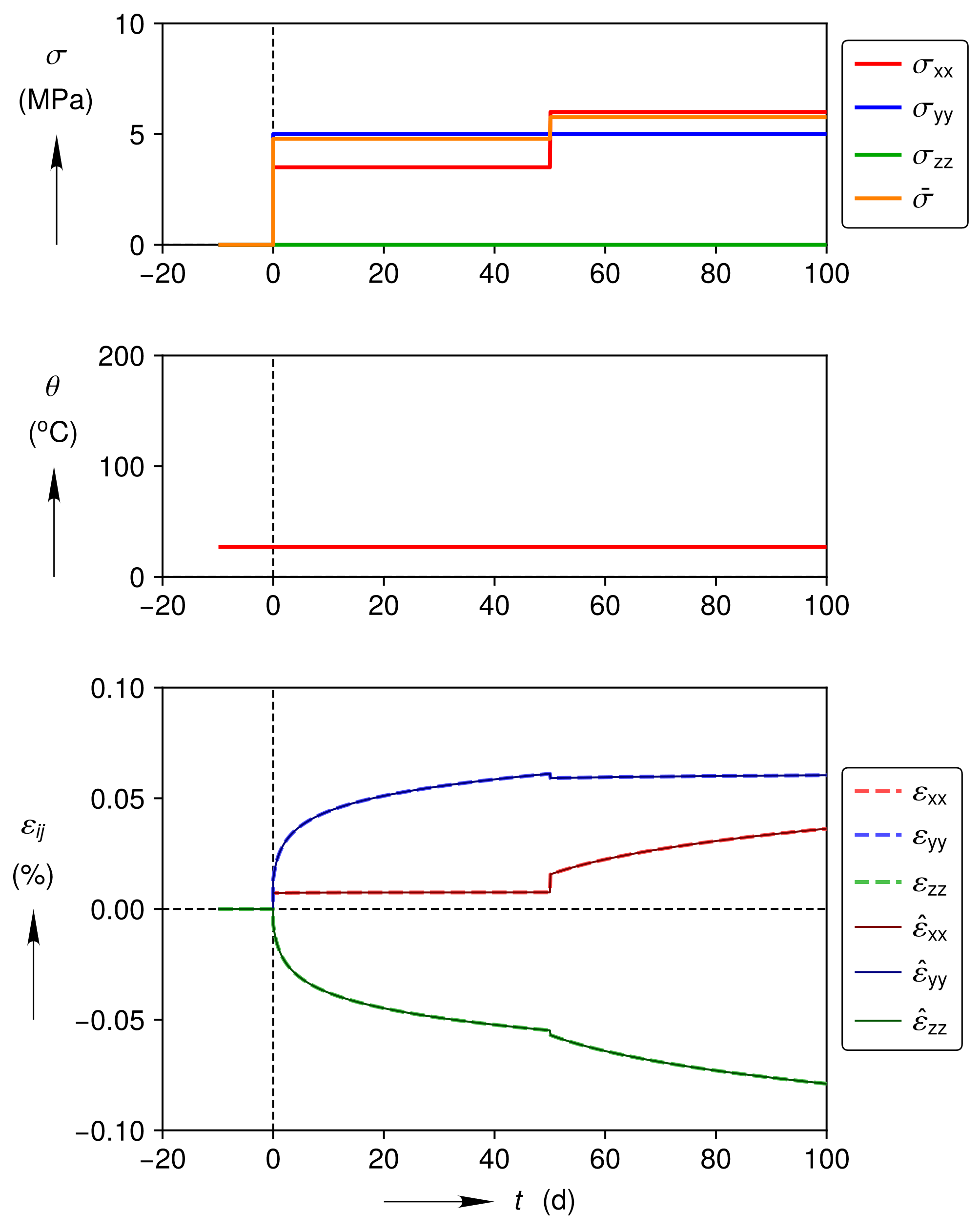
Fig. 4.104 Unequal Biaxial Compression Verification Test

The applied stress and temperature histories for the test are shown in the top two plots in Fig. 4.104. The test begins with a stress free hold period for 10 days. At \(t=0\), \(\sigma_{\text{xx}}\) is increased to 3.5~MPa, \(\sigma_{\text{yy}}\) is increased to 5~MPa, and \(\sigma_{\text{zz}}\) is held at zero. In this stress state, \(\psi=13.0^\circ\) and the intermediate principal stress is \(\sigma_{\text{xx}}\). The intermediate principal strain rate \(\dot{\varepsilon}_{\text{xx}}\approx0\) and \(\dot{\varepsilon}_{\text{yy}}\approx-\dot{\varepsilon}_{\text{zz}}\) because the flow rule (4.94) causes \(\dot{\varepsilon}^{\text{vp}}\) to be coaxial with the flow potential normal \(n_{ij}\), and \(n_{ij}\) is nearly horizontal at \(\phi=13.0^\circ\) in Calibration 3B (see Fig. 4.99). At \(t=50\), \(\sigma_{\text{xx}}\) is increased to 6.0~MPa, while the other stresses remain fixed. The sharp increase in \(\sigma_{\text{xx}}\) causes a step change in elastic strain that is visible because the viscoplastic strains are small at these low values of \(\bar{\sigma}\). In this stress state, \(\psi=21.1^\circ\) and the intermediate principal stress is \(\sigma_{\text{yy}}\). Accordingly, \(\dot{\varepsilon}_{\text{yy}}\approx0\) and \(\dot{\varepsilon}_{\text{xx}}\approx-\dot{\varepsilon}_{\text{zz}}\). If one looks more closely, however, \(\dot{\varepsilon}_{\text{yy}}\) is slightly positive and \(\dot{\varepsilon}_{\text{xx}}> -\dot{\varepsilon}_{\text{zz}}\) because \(\psi=21.1^\circ\) is beginning to approach the corner of the Tresca hexagon (see again Fig. 4.99).

In summary, the numerical and analytical solutions for the total strain match very well throughout the test, which verifies:

• Linear elasticity under unequal biaxial compression

• Viscoplastic strain evolution for \(\psi=13.0^\circ\) and a subsequent change to \(\psi=21.1^\circ\)

• Transient strain accumulation dominated by transient strain limit mechanism 0

• Steady-state strain accumulation dominated by mechanism 0.

4.21.4. User Guide

BEGIN PARAMETERS FOR MODEL MD_VISCOPLASTIC
  # Elastic constants
  YOUNGS MODULUS  = <real>
  POISSONS RATIO  = <real>
  SHEAR MODULUS   = <real>
  BULK MODULUS    = <real>
  LAMBDA          = <real>
  TWO MU          = <real>
  # Steady-state creep parameters
  A0              = <real> (0.0)
  A1              = <real> (0.0)
  A2              = <real> (0.0)
  Q0oR            = <real> (0.0)
  Q1oR            = <real> (0.0)
  Q2oR            = <real> (0.0)
  n0              = <real> (0.0)
  n1              = <real> (0.0)
  n2              = <real> (0.0)
  sigma_g         = <real>
  B0              = <real> (0.0)
  B1              = <real> (0.0)
  B2              = <real> (0.0)
  q               = <real> (0.0)
  # Transient creep parameters
  K0              = <real> (0.0)
  K1              = <real> (0.0)
  c0              = <real> (0.0)
  c1              = <real> (0.0)
  m0              = <real> (0.0)
  m1              = <real> (0.0)
  alpha_h         = <real> (0.0)
  alpha_r         = <real> (0.0)
  beta_h          = <real> (0.0)
  beta_r          = <real> (0.0)
  # Other parameters
  alpha           = <real> (0.0)
  a               = <real> (1000.0)
  # Numerical implementation parameters
  _chi            = <real> (2.0)
  _sigma_min      = <real> (1e-10 * SHEAR_MODULUS)
  _sqrt_omega_max = <real> (1e-11)
  _xi             = <real> (1e-4)
  _gamma          = <real> (0.1)
  _k_max          = <real> (100)
  _j_max          = <real> (10)
END [PARAMETERS FOR MODEL MD_VISCOPLASTIC]

Output variables available for this model are listed in Table 4.32.

Table 4.32 State Variables for MD_VISCOPLASTIC Model

Name	Description
EQ_TR_STRAIN	equivalent transient viscoplastic strain, \(\bar{\varepsilon}^\mathrm{tr}\)
EQ_VP_STRAIN	equivalent viscoplastic strain, \(\bar{\varepsilon}^\mathrm{vp}\)
EQ_STRESS	equivalent stress, \(\bar{\sigma}\)
VP_RATE_SCALE_FACTOR	viscoplastic rate scale factor, \(s\)

---

[1]

Darrell E Munson and PR Dawson. Constitutive model for the low temperature creep of salt (with application to WIPP). Technical Report SAND79-1853, Sandia National Laboratories, Albuquerque, NM, 1979.

[2]

Darrell E Munson and PR Dawson. Transient creep model for salt during stress loading and unloading. Technical Report SAND82-0962, Sandia National Laboratories, Albuquerque, NM, 1982.

[3]

Darrell E Munson, Arlo F Fossum, and Paul E Senseny. Advances in resolution of discrepancies between predicted and measured in situ WIPP room closures. Technical Report SAND88-2948, Sandia National Laboratories, Albuquerque, NM, 1989.

[4] (1,2,3,4)

Benjamin Reedlunn. Enhancements to the munson-dawson model for rock salt. Technical Report SAND2018-12601, Sandia National Laboratories, Albuquerque, NM, 2018.

[5]

W.F. Hosford. A generalized isotropic yield criterion. Journal of Applied Mechanics, 39:607–609, 1972.

[6]

Benjamin Reedlunn, James Bean, John Wilkes, and John Bignell. Simulations of criticality control overpack container compaction at the waste isolation pilot plant. Technical Report SAND2019-3106 O, Sandia National Laboratories, Albuquerque, NM, 2019.

[7]

W. M. Scherzinger. A return mapping algorithm for isotropic and anisotropic plasticity models using a line search method. Computer Methods in Applied Mechanics and Engineering, 317:526–553, 2017.