4.23. Hyperelastic Damage Model

4.23.1. Theory

The hyperelastic damage model is an isotropic, strain rate and temperature independent continuum damage formulation. In this case, the specific form is that discussed by Holzapfel [[1]] and proposed primarily for particulate reinforced (filled) rubber-like materials exhibiting the so called Mullins effect. Specifically, this model utilizes a Kachanov-like effective stress concept to propose an effective Helmholtz free energy, \(W\), of the form

\[W=\left(1-\zeta\right)W_0\left(C_{ij}\right),\]

in which \(\zeta=\left[0,1\right]\) is the isotropic damage variable and \(W_0\) is the Helmholtz free energy of the undamaged material and \(C_{ij}\) is the right Cauchy-Green tensor (\(C_{ij}=F_{ki}F_{kj}\) with \(F_{ij}\) the deformation gradient). The free energy expression of the neo-Hookean model (Section 4.5) is used to describe the undamaged strain energy and is given as,

\[W_0\left(C_{ij}\right)=\frac{1}{2}K\left[\frac{1}{2}\left(J^2-1\right)-\ln J\right]+\frac{1}{2}\mu\left(\bar{C}_{kk}-3\right),\]

with \(K\) and \(\mu\) the bulk and shear moduli, \(J\) the determinant of the deformation gradient and \(\bar{C}_{kk}\) the isochoric part of the deformation – \(\bar{C}_{ij}=\bar{F}_{ki}\bar{F}_{kj}\) and \(\bar{F}_{ij}=J^{-1/3}F_{ij}\). In the undamaged configuration, the second Piola-Kirchoff stress, \(S^0_{ij}\), is the energetic conjugate of the right Cauchy-Green strain such that

\[S^0_{ij}=2\frac{\partial W_0}{\partial C_{ij}},\]

leading to a damaged stress of the form,

\[S_{ij}=\left(1-\zeta\right)S^0_{ij}.\]

To describe the softening process, two damage related variables are needed. The first is the previously mentioned smooth, continuous effective damage variable, \(\zeta\), while the second is the so-called discontinuous damage variable, \(\alpha\). In essence, this second variable may be considered to be the maximum strain energy in the undamaged material throughout the entire loading history. This statement may be expressed as,

(4.111)\[\alpha=\max_{s\in\left[0,t\right]}W_{0}\left(s\right),\]

in which \(s\) is a history variable representing any time in the loading history and the dependence on \(s\) in (4.111) is used to indicate the loading history and not an explicit dependence on time or strain rate. The two damage terms are related by assuming \(\zeta=\zeta\left(\alpha\right)\). To ascertain this dependence, it is noted that \(\zeta\left(0\right)=0\) and \(\zeta\left(\infty\right)=1\) the former explicitly stating that the material is initially undamaged and the latter noting in the limit the material is completely damaged the strain energy will go to \(\infty\). These observations lead to an expression of the form,

(4.112)\[\zeta\left(\alpha\right)=\zeta_{\infty}\left[1-\exp\left(-\alpha/\tau\right)\right],\]

with \(\tau\) being a constant referred to as the damage saturation parameter and \(\zeta_{\infty}\) being the maximum value of the damage parameter that may be achieved.

The evolution of the damage process is governed by a so-called damage function, \(f\left(C_{ij},\alpha\right)\) (analogous to the yield function in plasticity), postulated as,

\[f\left(C_{ij},\alpha\right) = \phi\left(C_{ij}\right)-\alpha,\]

where \(\phi\) is the thermodynamic driving of the damage process. In this case, the thermodynamic conjugate of the damage variable \(\zeta\) is the undamaged strain energy, \(W_0\), such that \(\phi\left(C_{ij}\right)=W_0\left(C_{ij}\right)\). By enforcing the consistency condition during damage (\(\dot{f}=0\)), it can be shown that,

\[\dot{\alpha}=\dot{\phi}=\frac{\partial W_0}{\partial C_{ij}}\dot{C}_{ij}=\frac{1}{2}S^0_{ij}\dot{C}_{ij}.\]

4.23.2. Implementation

For the hyperelastic damage model, the first step is to calculate the undamaged second Piola-Kirchoff stress, \(S^{0\left(n+1\right)}_{ij}\) of the current \(\left(n+1\right)^{th}\) time step. To this end, the deformation gradient, \(F^{\left(n+1\right)}_{ij}\), is calculated based on the input stretch, \(V^{\left(n+1\right)}_{ij}\), and rotation, \(R^{\left(n+1\right)}_{ij}\), tensors via the polar decomposition. The second Piola-Kirchoff stress may then be determined as,

\[S^{0\left(n+1\right)}_{ij}=\left[\frac{1}{2}K\left(\left(J^{\left(n+1\right)}\right)^2-1\right)I_{il} +\mu \left(J^{\left(n+1\right)}\right)^{-2/3}\left(C^{\left(n+1\right)}_{il}-\frac{1}{3}C^{\left(n+1\right)}_{kk}I_{il}\right)\right]\left(C^{\left(n+1\right)}_{jl}\right)^{-1}.\]

To determine the damage state, the undamaged strain energy \(W^{\left(n+1\right)}_0\), is first calculated as,

\[W^{\left(n+1\right)}_0=\frac{1}{2}K\left(\frac{1}{2}\left(\left(J^{\left(n+1\right)}\right)^2-1\right)-\ln J^{\left(n+1\right)}\right) +\frac{1}{2}\mu\left[\left(J^{\left(n+1\right)}\right)^{-2/3}C^{\left(n+1\right)}_{kk}-3\right].\]

The current discrete damage variable, \(\alpha^{\left(n+1\right)}\), may then be determined via,

\[\alpha^{\left(n+1\right)}=\max\left[\alpha^{\left(n\right)},W_0^{\left(n+1\right)}\right],\]

so that the current continuous damage variable, \(\zeta^{\left(n+1\right)}\), is,

\[\zeta^{\left(n+1\right)}=\zeta_{\infty}\left[1-\exp\left(\alpha^{\left(n+1\right)}/\tau\right)\right].\]

Finally, these expressions lead to an unrotated Cauchy stress of the form,

\[T_{ij}^{\left(n+1\right)}=\frac{1}{J^{\left(n+1\right)}}\left(1-\zeta^{\left(n+1\right)}\right) R^{\left(n+1\right)}_{ki}F^{\left(n+1\right)}_{km}S^{0\left(n+1\right)}_{mn}F^{\left(n+1\right)}_{rn}R^{\left(n+1\right)}_{rj}.\]

4.23.3. Verification

Given the hyperelastic formulation of the hyperelastic damage model, it is possible to find closed form solutions for simple loadings. Two such instances (uniaxial strain and simple shear) are considered here to evaluate and verify the response of this implementation. In this case, the results explored here are extensions of the neo-Hookean verification tests previously discussed in Section 4.5.3 and [[2]]. One set of material properties was used for all tests and they are given in Table 4.34. The damage parameters are taken from [[1]].

Table 4.34 The material properties for the hyperelastic damage model used for both the uniaxial and simple shear tests.

Name	Description
\(K\)	0.5 MPa	\(\mu\)	0.375 MPa
\(\zeta_{\infty}\)	0.8	\(\tau\)	0.3 MPa

4.23.3.1. Uniaxial Strain

First, utilizing a displacement condition corresponding to uniaxial strain results in a deformation gradient of the form,

(4.113)\[F_{ij}=\lambda\delta_{1i}\delta_{1j} + \delta_{2i}\delta_{2j}+\delta_{3i}\delta_{3j}.\]

As the undamaged material is neo-Hookean, it is noted that the under these loading conditions the stress field is found by evaluating relation (4.10) and may be written as

\[\begin{split}\sigma^0_{11} & = \frac{1}{2}K\left(\lambda-\frac{1}{\lambda}\right)+\frac{2}{3}\mu\left(\lambda^2-1\right)\lambda^{-5/3}, \nonumber \\ \sigma^0_{22}=\sigma^0_{33} & =\frac{1}{2}K\left(\lambda-\frac{1}{\lambda}\right)-\frac{1}{3}\mu\left(\lambda^2-1\right)\lambda^{-5/3}, \\ \sigma^0_{12}=\sigma^0_{23}=\sigma^0_{31}& = 0 \nonumber.\end{split}\]

The damaged, effective stresses are then simply \(\sigma_{ij}=\left(1-\zeta\right)\sigma^0_{ij}\) and the problem reduces to the determination of \(\zeta\). In this case, given the deformation gradient in (4.113), \(J=\lambda\) and

\[W_0=\frac{1}{2}K\left[\frac{1}{2}\left(\lambda^2-1\right)-\ln\lambda\right]+\frac{1}{2}\mu\left[\lambda^{-2/3}\left(\lambda^2+2\right)-3\right].\]

During loading, \(\alpha=W_0\) while during unloading \(\alpha=W_0\left(\lambda^{\text{max}}\right)\) and \(\zeta\) can be determined from (4.112).

Both the corresponding analytical and numerical solutions are presented in Fig. 4.113 for a complete loading and unloading cycle. Note, the damage parameter, \(\zeta\), increases during loading but remains constant during unloading verifying the irreversibility of the proposed model.

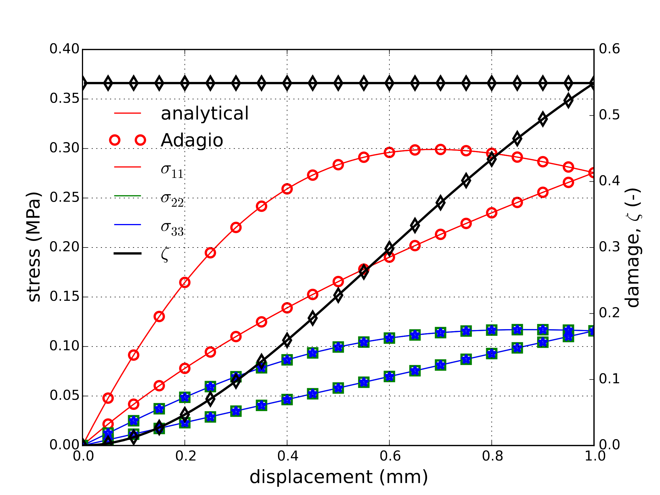
Fig. 4.113 Analytical and numerical results of the stress and damage state for the uniaxial stretch case.

4.23.3.2. Simple Shear

For the simple shear case, a deformation gradient of the form,

\[F_{ij}=\delta_{ij}+\gamma\delta_{1i}\delta_{2j},\]

is prescribed. Again, from the neo-Hookean model definitions the undamaged stresses may be determined via (4.10) and noting this is a volume preserving definition (\(J=1\)) leading to expressions of the form,

\[\begin{split}\sigma^0_{11} & = \frac{2}{3}\mu\gamma^2, \nonumber \\ \sigma^0_{22}=\sigma_{33} & = -\frac{1}{3}\mu\gamma^2, \nonumber \\ \sigma^0_{12} & = \mu\gamma, \\ \sigma^0_{23}=\sigma^0_{31} & = 0. \nonumber\end{split}\]

In this case, the undamaged strain energy is simply,

\[W_0=\frac{1}{2}\mu\gamma^2,\]

and \(\zeta\) may be evaluated via (4.112). The effective stresses are then \(\sigma_{ij}=\left(1-\zeta\right)\sigma^0_{ij}\)

Both the corresponding analytical and numerical solutions are presented in Figure. Fig. 4.114 for a complete loading and unloading cycle. Note, the damage parameter, \(\zeta\), increases during loading but remains constant during unloading given the irreversible form of the damage process.

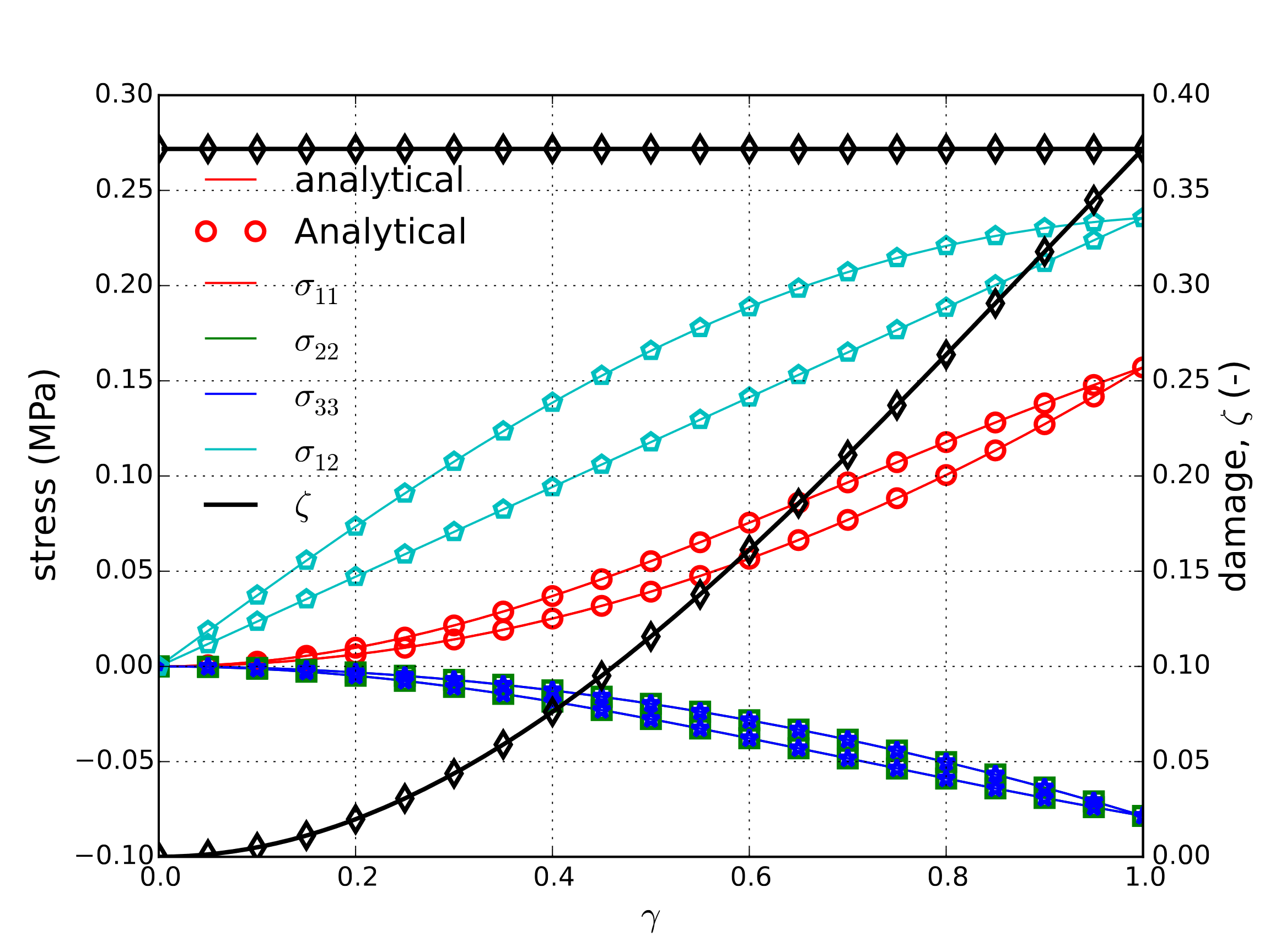
Fig. 4.114 Analytical and numerical results of the stress and damage state for the simple shear case.

4.23.4. User Guide

BEGIN PARAMETERS FOR MODEL HYPERELASTIC_DAMAGE
  #
  # Elastic constants
  #
  YOUNGS MODULUS = <real>
  POISSONS RATIO = <real>
  SHEAR MODULUS  = <real>
  BULK MODULUS   = <real>
  LAMBDA         = <real>
  TWO MU         = <real>
  #
  DAMAGE MAX        = <real>
  DAMAGE SATURATION = <real>
END [PARAMETERS FOR MODEL HYPERELASTIC_DAMAGE]

Output variables available for this model are listed in Table 4.35. For information about the hyperelastic damage model, consult [[1]].

Table 4.35 State Variables for HYPERELASTIC DAMAGE Model

Name	Description
DAMAGE	continuous isotropic damage variable, \(\zeta\)
ALPHA	discontinuous damage variable, \(\alpha\)
PRESSURE	reference undamaged tensile pressure, \(\left(1/3\right)\left(1-\zeta\right)S_{kk}\)

---

[1] (1,2,3)

G. A. Holzapfel. Nonlinear Solid Mechanics: A Continuum Approach For Engineering. John Wiley & Sons, Ltd, 2000.

[2]

W.M. Scherzinger and D.C. Hammerand. Testing of constitutive models in LAME. Technical Report SAND2007-5872, Sandia National Laboratories, Albuquerque, NM, September 2007. \href http://infoserve.sandia.gov/sand_doc/2007/075872.pdfpdf.