4.31. Orthotropic Rate Model

4.31.1. Theory

The orthotropic rate model is an improved version of the orthotropic crush model [[1]] that incorporates anisotropic elasticity, strain-rate dependence, and the ability to define the material coordinate system. The specific form of this model is motivated by metallic honeycombs and the material coordinate system is usually given in terms of \(T,~L,\) and \(W\) directions. These directions correspond to the strong (\(T\)) and ribbon (\(L\)) axes depicted in Fig. 4.134. The third component of the coordinate system, \(W\), is the weak direction and is simply the cross-product of the other two directions.

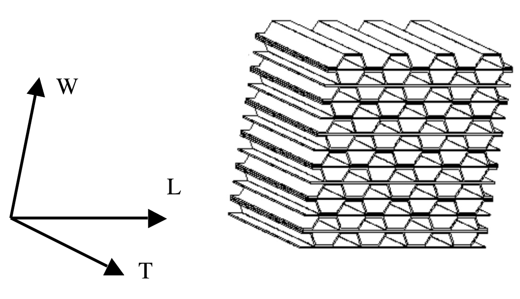
Fig. 4.134 Orientation of the T, L and W vectors for 38 pc aluminum honeycomb.

In terms of expected response, and similar to the orthotropic crush model, the deformation is split into two regimes – uncompacted and compacted. Unlike the crush model, the state of compaction is not determined by the determinant of the deformation gradient but is instead a function of the engineering (not logarithmic) volume strain, \(\varepsilon_{\text{V}}\). The degree of compaction, \(\alpha\), is therefore defined as,

\[\alpha=\min_{t>0}\left(\frac{V_0-V\left(t\right)}{V_0}\right)=1-\frac{\min_{t>0}V\left(t\right)}{V_0}=-\min_{t>0}\varepsilon_{\text{V}}\left(t\right),\]

with \(V\left(t\right)\) and \(V_0\) being the current and original volume of the material. Complete compaction occurs at a user specified value, \(\alpha_{\text{comp}}\).

Prior to complete compaction, the elastic stiffness, \(\mathbb{C}_{ijkl}\), is taken to exhibit orthotropic symmetry and depends on the compaction state of the material, \(\mathbb{C}_{ijkl}=\mathbb{C}_{ijkl}\left(\alpha\right)\). In the material frame and in Voigt notation, this stiffness is represented as,

(4.144)\[\begin{split}\left[\mathbb{C}\left(\alpha\right)\right] = \begin{bmatrix} E_{TTTT}\left(\alpha\right) & E_{TTLL}\left(\alpha\right) & E_{TTWW}\left(\alpha\right) & 0 & 0 & 0 \\ \\ E_{TTLL}\left(\alpha\right) & E_{LLLL}\left(\alpha\right) & E_{LLWW}\left(\alpha\right) & 0 & 0 & 0 \\ \\ E_{TTWW}\left(\alpha\right) & E_{LLWW}\left(\alpha\right) & E_{WWWW}\left(\alpha\right) & 0 & 0 & 0 \\ \\ 0 & 0 & 0 & G_{TLTL}\left(\alpha\right) & 0 & 0 \\ \\ 0 & 0 & 0 & 0 & G_{LWLW}\left(\alpha\right) & 0 \\ \\ 0 & 0 & 0 & 0 & 0 & G_{WTWT}\left(\alpha\right) \end{bmatrix}.\end{split}\]

Once the material is completely compacted, the elastic stiffness is taken to be isotropic and the evolution of the initially orthotropic components (\(E_{TTTT}\left(\alpha=0\right)=E^0_{TTTT}\)) to final isotropic, compacted coefficients (\(E_{TTTT}\left(\alpha=\alpha_{\text{comp}}\right)=\lambda+2\mu\) with \(\lambda\) and \(2\mu\) being Lam'{e}’s constant and the shear modulus) is given via a common user-defined scaling function, \(f_E\left(\alpha\right)\). The mechanical stiffness coefficients then scale as,

(4.145)\[E_{TTTT}\left(\alpha\right)=E_{TTTT}^0+\left(\lambda+2\mu-E_{TTTT}^0\right)f_E\left(\alpha\right),\]

for the volumetric diagonal terms (\(E_{TTTT},~E_{LLLL},~E_{WWWW}\)),

(4.146)\[E_{TTLL}\left(\alpha\right)=E_{TTLL}^0+\left(\lambda-E_{TTLL}^0\right)f_E\left(\alpha\right),\]

for the off-diagonal terms (\(E_{TTLL},~E_{TTWW},~E_{LLWW}\)) and

\[G_{TLTL}\left(\alpha\right)=G_{TLTL}^0+\left(2\mu-G_{TLTL}^0\right)f_E\left(\alpha\right)\]

for the shear terms. From these relations, it is obvious that \(f_E\left(\alpha\right)\) should be bounded such that \(0\leq f_E\left(\alpha\right)\leq 1\) with \(f_E\left(0\right)=0\) and \(f_E\left(\alpha_{\text{comp}}\right)=1\).

As was mentioned earlier, the deformation and model response may be readily split between two regimes – the uncompacted and compacted. The behavior during the latter regime is simpler and is assumed to be that of an isotropic elastic-perfectly plastic material characterized by the elastic coefficients (\(\lambda,~2\mu\)) and yield stress (\(\sigma_y\)). During the uncompacted regime the deformation is more complex and typical responses may include elastic bending of cell structures, buckling of cell walls, or densification (see the text of Gibson and Ashby [[2]] for a complete discussion of these and other mechanisms). In this formulation, however, none of these deformation modes are explicitly modeled. Instead, the response is defined via six independent yield functions (one for each stress component in the material coordinate system), \(\phi_{\beta\gamma}\), that are a function of the corresponding stress, the compaction state, and the current strain rate, \(\dot{\bar{\varepsilon}}=\sqrt{d_{ij}d_{ij}}\). Here, \(d_{ij}\) is the unrotated rate of deformation in the global (\(X,Y,Z\)) coordinate system and \(\beta\) and \(\gamma\) are being used as subscripts to denote variables in the material coordinate system.

The six yield functions are,

\[\begin{split}\begin{split} \phi_{LL} & = \sigma_{LL}-f_{LL}\left(\alpha\right) h\left(\dot{\bar{\varepsilon}}\right)\\ \phi_{TT} & = \sigma_{TT}-f_{TT}\left(\alpha\right) h\left(\dot{\bar{\varepsilon}}\right)\\ \phi_{WW} & = \sigma_{WW}-f_{WW}\left(\alpha\right) h\left(\dot{\bar{\varepsilon}}\right)\\ \phi_{LT} & = \sigma_{LT}-f_{LT}\left(\alpha\right) h\left(\dot{\bar{\varepsilon}}\right)\\ \phi_{TW} & = \sigma_{TW}-f_{TW}\left(\alpha\right) h\left(\dot{\bar{\varepsilon}}\right)\\ \phi_{WL} & = \sigma_{WL}-f_{WL}\left(\alpha\right) h\left(\dot{\bar{\varepsilon}}\right) \end{split},\end{split}\]

with \(\sigma_{\beta\gamma}\) being the current symmetric Cauchy stresses in the material coordinate system, \(f_{\beta\gamma}\) are user specified hardening functions defining the maximum stress in that direction for a given compaction state and \(h\left(\dot{\bar{\varepsilon}}\right)\) is the strain rate sensitivity function that is common to all the yield functions. With these forms, it is evident that the definition of the different hardening functions dictates the model response through the uncompacted regime. All (or none) of the aforementioned deformation mechanisms may be captured by the appropriate definition of those functions. As such, the response is dictated by the desire of the analyst and appropriate selection of the elastic scaling, hardening, and strain rate sensitivity function – \(f_E\left(\alpha\right),~f_{\beta\gamma}\left(\alpha\right)\), and \(h\left(\dot{\bar{\varepsilon}}\right)\).

4.31.2. Implementation

Unlike the orthotropic crush model, the rate variant considered here has couplings between the different directional strains and cannot be evaluate numerically as easily. Therefore, the orthotropic rate model is integrated using a hypoelastic formulation. As was discussed in the preceding section, the model is formulated in the \(T,~L,~W\) coordinate system and not the unrotated frame. Therefore, the first step before proceeding is to map strain and stress values from the unrotated to the material frame. To this end, an orthogonal rotation tensor \(\tilde{Q}_{ij}\) is constructed from user input vectors \(\hat{t}_i\) and \(\hat{l}_i\) defining the strong and ribbon directions, respectively. In this case, the \(~\tilde{\cdot}~\) is used to differentiate this tensor from that mapping between the rotated and unrotated configurations defined in (4.1). The stress and deformation rates in the material coordinate system, \(\tilde{\sigma}_{ij}\) and \(\tilde{d}_{ij}\), are determined via,

(4.147)\[\begin{split}\tilde{\sigma}^n_{ij}=\tilde{Q}_{ki}T^n_{kl}\tilde{Q}_{lj}, \\ \tilde{d}^{n+1}_{ij}=\tilde{Q}_{ki}d^{n+1}_{kl}\tilde{Q}_{lj},\end{split}\]

where \(T^n_{ij}\) and \(d^{n+1}_{ij}\) are the unrotated stress and deformation rates, respectively. For convenience, the remainder of this discuss will neglect the \(~\tilde{\cdot}~\) notation and all operations will be assumed to be in the material coordinate system unless specifically noted. Additionally, after a converged stress is achieved, the inverse mapping of (4.147) is used to determine \(T^{n+1}_{ij}\).

As the strain increment is fixed for a load step, kinematically defined variables such as \(\alpha^{n+1}\) and the strain rate, \(\dot{\bar{\varepsilon}}^{n+1}\), may first be determined. The latter term is defined as,

\[\dot{\bar{\varepsilon}}^{n+1}=\sqrt{d^{n+1}_{ij}d^{n+1}_{ij}},\]

with \(d^{n+1}_{ij}\) being the strain rate in the global coordinate system. For the former, it must first be noted that the engineering, \(\varepsilon_{\text{V}}\), and logarithmic, \(\varepsilon_{kk}\), volumetric strains are related via \(\varepsilon_{\text{V}}=\exp{\left(\varepsilon_{kk}\right)}-1\). The current state of compaction is then given as,

\[\alpha^{n+1}=1-\hat{\varepsilon}^{n+1}_{V},\]

where \(\hat{\varepsilon}^{n+1}_{V}=\min\left[\hat{\varepsilon}^n_{V},\exp{\left(\varepsilon^{n+1}_{kk}\right)}\right]\).

The material response has two distinct regimes. As discussed in the corresponding theory section, the compacted material behaves as an elastic-plastic material. Such a response and the corresponding numerical analysis has been described in Section 4.7.2. As such, it will not be further presented here and instead the focus is on the behavior during the uncompacted stages.

Earlier, it was mentioned that the response during the compaction process is dictated by three functions – the elastic scaling, hardening, and strain rate sensitivity. These three expressions are dependent on the state of compaction and strain rate. As those kinematic properties have already been calculated, the values of \(f_{E}^{n+1}=f_{E}\left(\alpha^{n+1}\right)\), \(f^{n+1}_{ij}=f_{ij}\left(\alpha^{n+1}\right)\), and \(h^{n+1}=h\left(\dot{\bar{\varepsilon}}^{n+1}\right)\) may easily be calculated. In the remainder of this section, the functional dependencies of these terms will not be explicitly presented for ease and brevity. Similarly, the superscript \(n+1\) will be dropped and it should be assumed that unless specifically denoted the variable is evaluated at the \(n+1\) step. With \(f_E\) (and \(f_E^n\)) defined, the elastic stiffness, \(\mathbb{C}_{ijkl}\) and \(\mathbb{C}_{ijk}^n\), and compliance, \(\mathbb{S}_{ijkl}\) and \(\mathbb{S}_{ijkl}^n\), tensors may also be calculated.

To determine the updated material state, the change in elastic stiffness (associated with the change in compaction) must be determined. To this end,

\[\hat{\sigma}_{ij}^n=\mathbb{C}_{ijkl}\varepsilon^{\text{e}-n}_{kl}\]

where

\[\varepsilon^{\text{e}-n}_{ij}=\mathbb{S}^n_{ijkl}\sigma_{kl}^n.\]

In the previous two relations, it is noted that the respective mechanical tensors are determined at different load steps thus leading to the altered stress state. The tensor \(\sigma_{ij}^n\) refers to the stress determined and stored from the previous load step while \(\hat{\sigma}_{ij}^n\) incorporates the change in mechanical stiffness. A trial stress state may be calculated as,

\[\sigma^{tr}_{ij}=\hat{\sigma}^n_{ij}+\mathbb{C}_{ijkl}d\varepsilon^{\text{e}-tr}_{kl},\]

with the trial elastic strain increment, \(d\varepsilon^{\text{e}-tr}_{ij}\) being that of the total strain increment, \(d_{ij}\Delta t\). The flow (yield) functions, \(f_{ij}^{tr}\), are then calculated. If all \(f_{ij}^{tr}<0\), the solution is elastic and the trial state is accepted. On the other hand, if any \(f_{ij}^{tr}>0\) a correction scheme is needed. This poses a more complex problem than in the orthotropic crush model given the multiple (six) yield surfaces.

To perform the plastic correction, an approach similar in principle to the return-mapping schemes heavily used in metal plasticity (e.g. Section 4.7.2). Here, however, there is no internal state variable and associated evolution equations to evolve the state. Instead, in this case the elastic strain is iterated over until all the yield conditions are satisfied. Specifically, for the \(k\)-th iteration, the stress is calculated as

\[\sigma^k_{ij}=\hat{\sigma}_{ij}^n+\mathbb{C}_{ijkl}d\varepsilon_{kl}^{\text{e}-k}.\]

Updated yield functions, \(f_{ij}^k\), are then calculated and the active flow directions (those with \(f_{ij}>0\)) determined. A tangent modulus is then constructed (essentially by turning off components corresponding to inactive directions) and a plastic flow tensor is determined using the tangent compliance and the value of the yield functions. The updated elastic strain increment, \(d\varepsilon_{ij}^{\text{e}-k+1}\), is then found by removing the calculated strain. This process is repeated until satisfaction of all the yield functions.

4.31.3. Verification

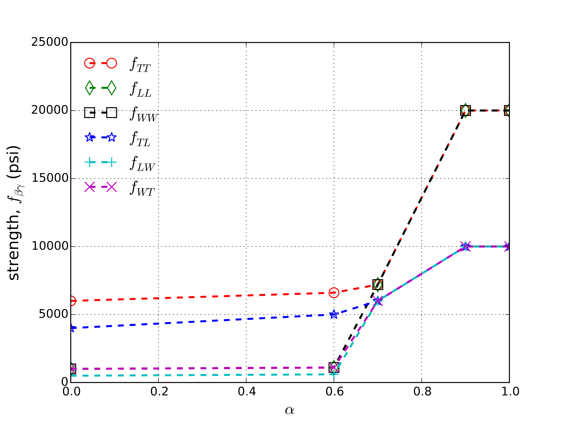
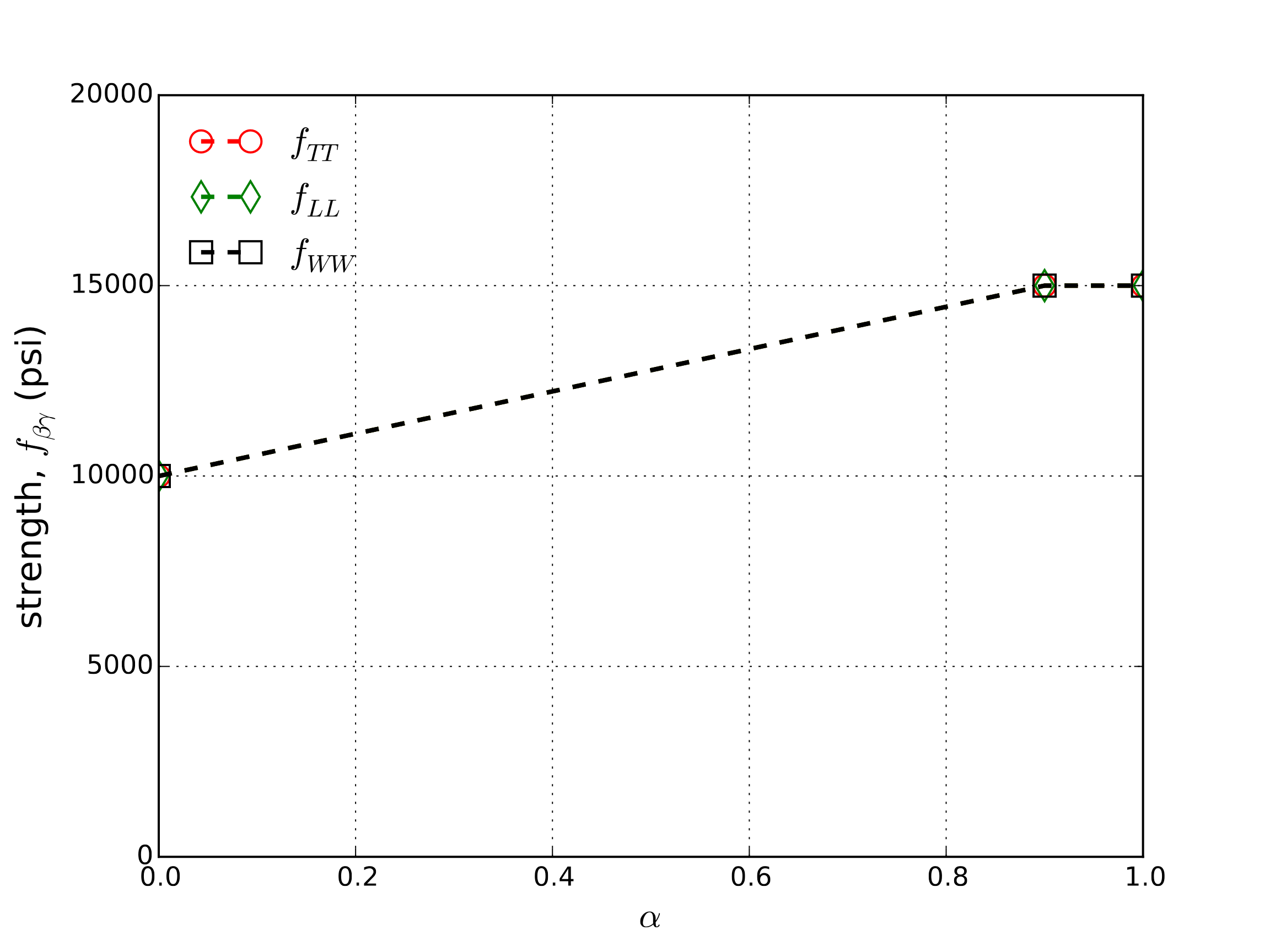
To verify the orthotropic crush model, a series of uniaxial compression tests are performed. Given the multiple salient features in this model (e.g. strain rate dependence, user-defined coordinate system), the test sequence is constructed to investigate and probe each of the different features to gain confidence in all of the anticipated capabilities. Additionally, the analyzed loading paths correspond to those in which the kinematics are fully prescribed. This is done so that analytical expressions may be found due to the strong coupling between the kinematics and constitutive response through the compaction state, \(\alpha\). The common model parameters used for these tests are given in Table 4.49 and the functional forms of the input strength/hardening curves, \(f_{\beta\gamma}\), are presented in Fig. 4.135. It is noted, however, that these properties will take various values during the verification tests to activate and deactivate different responses. Additionally, in Fig. 4.135, two sets of curves are given – the full, complex set of six distinct functions (Fig. 4.135a) and a simpler set (Fig. 4.135b). In the latter, only one curve common to the three diagonal strengths are shown. The other three strength functions are all set artificially high to enable the study of a simpler case.

Table 4.49 Material and model parameters for the orthotropic rate model used for verification

\(E^0_{TTTT}\)	2,322.0 ksi	\(E\)	4000.0 ksi
\(E^0_{TTLL}\)	485.8 ksi	\(\nu\)	0.3
\(E^0_{TTWW}\)	68.8 ksi	\(\sigma_y\)	15.0 ksi
\(E^0_{LLLL}\)	1,348.0 ksi	\(\hat{t}_x\)	1.0
\(E^0_{LLWW}\)	121.8 ksi	\(\hat{t}_y\)	0.0
\(E^0_{WWWW}\)	85.0 ksi	\(\hat{t}_z\)	0.0
\(G^0_{TLTL}\)	1,345.0 ksi	\(\hat{l}_x\)	0.0
\(G^0_{LWLW}\)	67.0 ksi	\(\hat{l}_y\)	1.0
\(G^0_{WTWT}\)	260.0 ksi	\(\hat{l}_z\)	0.0
\(h\left(\dot{\bar{\varepsilon}}\right)\)	1.0	\(f_{E}\left(\alpha\right)\)	\(\alpha\)

Complex case

Simple case

Fig. 4.135 Input strength/hardening curves, \(f_{\beta\gamma}\), for use in verification tests of the orthotropic rate model.

4.31.3.1. Uniaxial Strain - Isotropic

First, the response of the model with through a uniaxial strain loading is explored. In this case, the prescribed displacement is \(u_i=\hat{\lambda}\delta_{i1}\). For this initial study, isotropic elastic constants are assumed leading to \(E^0_L=E^0_{LLLL}=E^0_{TTTT}=E^0_{WWWW}=5,384.6\) ksi and \(E^0_T=E^0_{TTLL}=E^0_{TTWW}=E^0_{LLWW}=2,307.7\) ksi. These properties are chosen to match the compacted state and \(f_E\left(\alpha\right)\) is set to zero. In this way, the elastic properties are constant throughout loading. The shear moduli are scaled accordingly and the remaining properties are left unchanged from Table 4.49. In this case, the model response simplifies to

\[\alpha=-\hat{\lambda},\]

and

(4.148)\[\begin{split}\sigma_{11} = \left\{\begin{array}{cc} \hat{\sigma} & \hat{\sigma}\leq f_{TT}\left(\alpha\right) \\ f_{TT} & \hat{\sigma} > f_{TT}\left(\alpha\right) \end{array}\right.\end{split}\]

\[\begin{split}\sigma_{22} = \sigma_{33} = \left\{\begin{array}{cc} \lambda\ln\left(1+\hat{\lambda}\right) & \hat{\sigma}\leq f_{TT}\left(\alpha\right) \\ \frac{\lambda}{\lambda+2\mu}\sigma_{11} & \hat{\sigma} > f_{TT}\left(\alpha\right) \end{array}\right. ,\end{split}\]

where

\[\hat{\sigma}=\left(\lambda+2\mu\right)\ln\left(1+\hat{\lambda}\right).\]

The single linear hardening crush curve given in Fig. 4.135(b) is used for this analysis. The resulting stresses as a function of applied displacement, \(\hat{\lambda}\), are given in Fig. 4.136 and good agreement is noted.

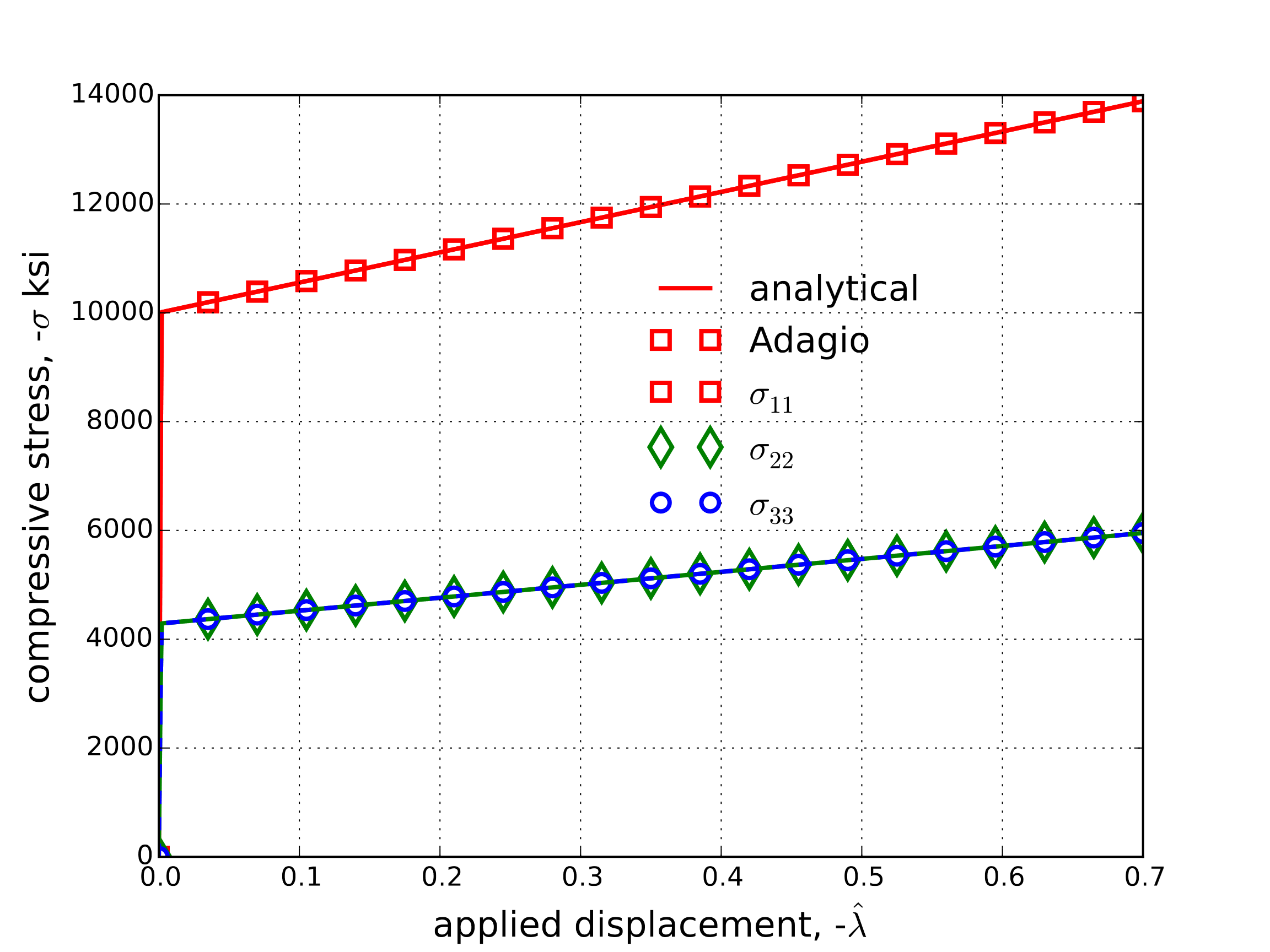
Fig. 4.136 Axial and off-axis stresses determined analytically and numerically via the orthotropic rate model with constant, isotropic elastic properties.

4.31.3.2. Uniaxial Strain - Orthotropic

The uniaxial problem described in the previous section is again studied – although this time using the orthotropic elastic properties listed in Table 4.49. To test the material coordinate system capabilities two cases are considered – essentially with the \(x_1\) axis aligned with the \(T\) and \(L\) axes. The first case corresponds to the definition of the \(\hat{t}_i\) and \(\hat{l}_i\) vectors in Table 4.49. Alternatively, the second case is defined by setting the \(L\) direction aligned with the \(x_1\) axis (\(\hat{l}_x=1.0,~\hat{l}_y=0.0,~\hat{l}_z=0.0\) and \(\hat{t}_x=0.0,~\hat{t}_y=0.0,~\hat{t}_z=1.0\)). The stress state evolutions determined via adagio and analytically for the two considered orientations are shown in Fig. 4.137(a) and Fig. 4.137(b), respectively. The analytical solutions are found in the same fashion as (4.148) with the moduli changed for the orthotropic case. Good agreement is observed.

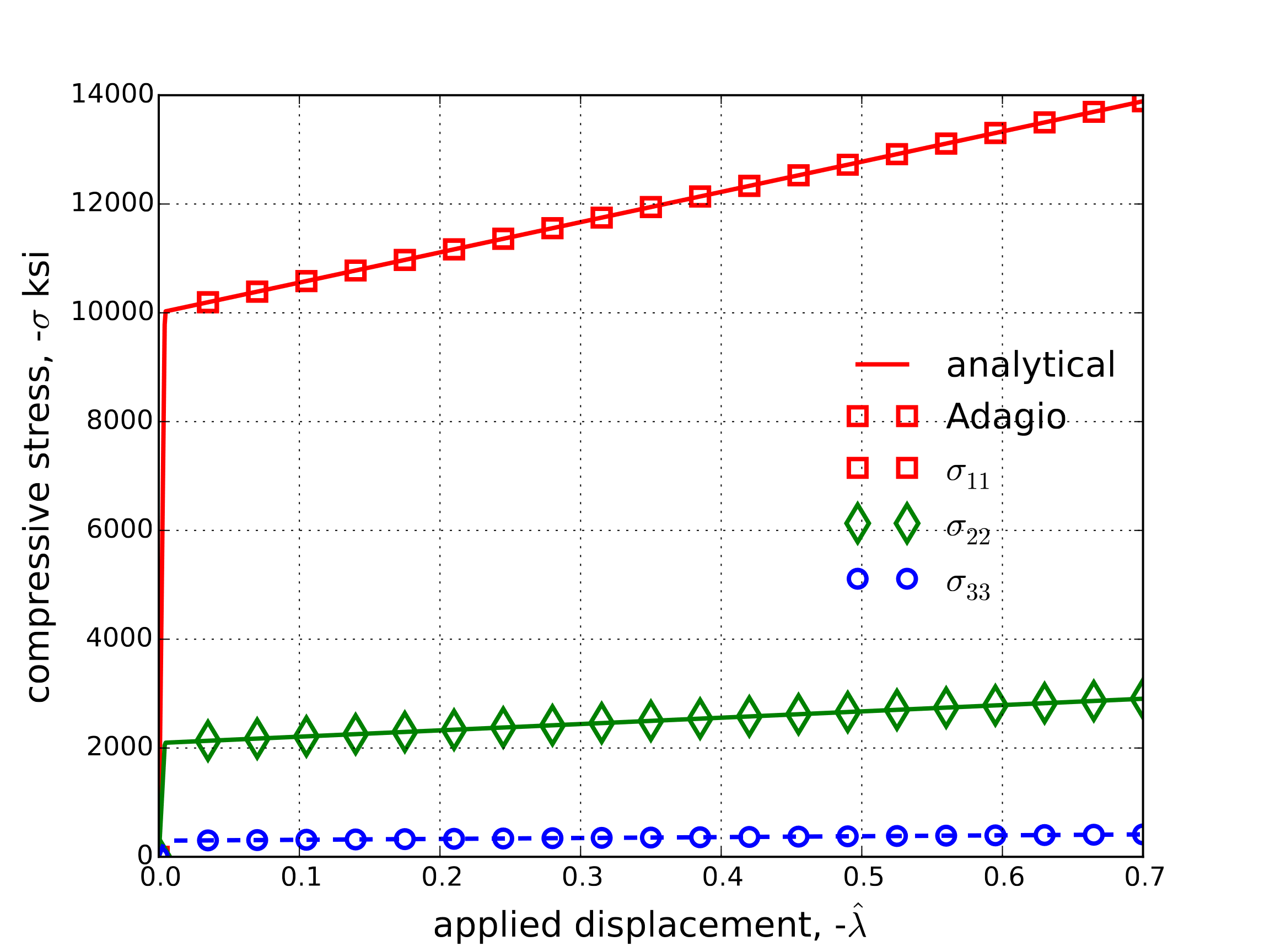Loading aligned with the T direction

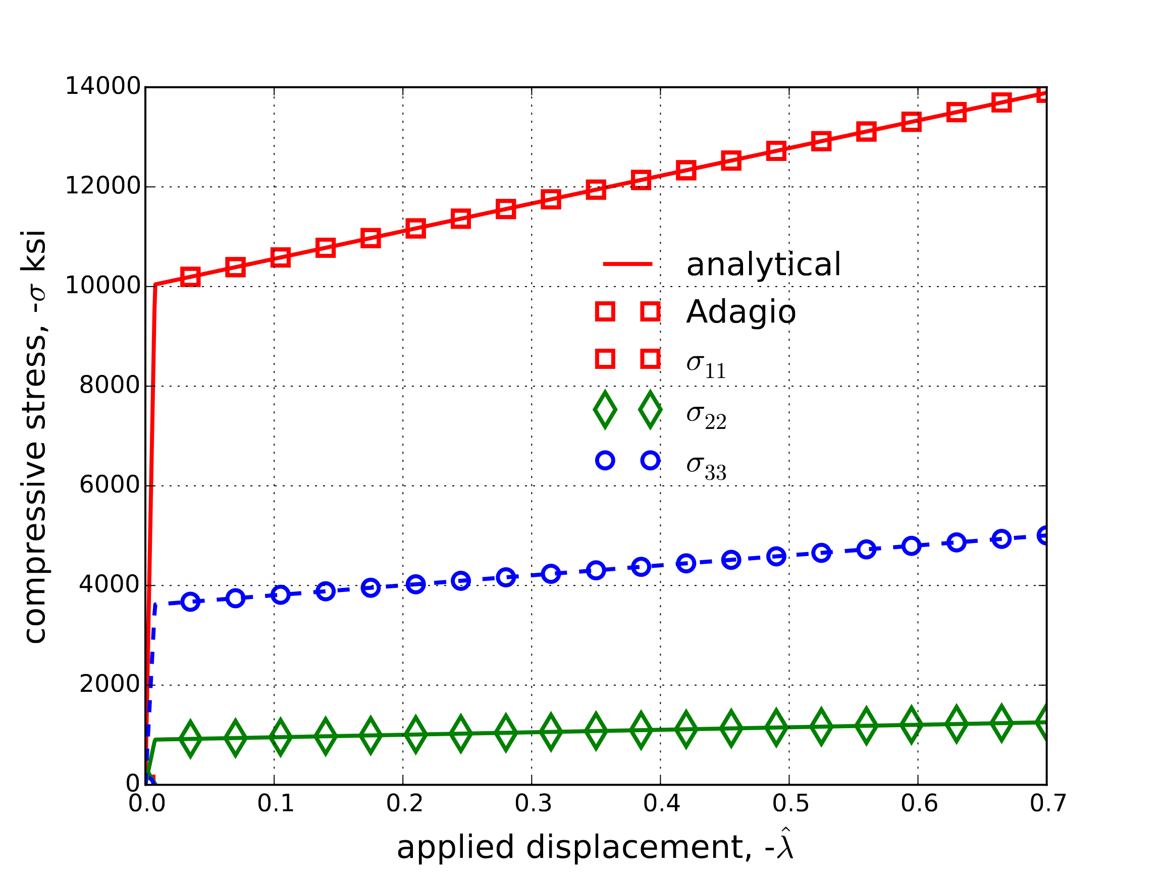Loading aligned with the W direction

Fig. 4.137 Axial and off-axis stresses determined analytically and numerically via the orthotropic rate model with constant, orthotropic elastic constants. The material coordinate systems is rotated in two different directions with the loading direction always aligned with \(x_1\)

4.31.4. User Guide

BEGIN PARAMETERS FOR MODEL ORTHOTROPIC_RATE
  #
  # Elastic constants
  #
  YOUNGS MODULUS = <real>
  POISSONS RATIO = <real>
  SHEAR MODULUS  = <real>
  BULK MODULUS   = <real>
  LAMBDA         = <real>
  TWO MU         = <real>
  #
  YIELD STRESS = <real>
  #
  MODULUS TTTT = <real>
  MODULUS TTLL = <real>
  MODULUS TTWW = <real>
  MODULUS LLLL = <real>
  MODULUS LLWW = <real>
  MODULUS WWWW = <real>
  MODULUS TLTL = <real>
  MODULUS LWLW = <real>
  MODULUS WTWT = <real>
  #
  TX = <real>
  TY = <real>
  TZ = <real>
  LX = <real>
  LY = <real>
  LZ = <real>
  #
  MODULUS FUNCTION = <string>
  RATE FUNCTION    = <string>
  #
  T FUNCTION  = <string>
  L FUNCTION  = <string>
  W FUNCTION  = <string>
  TL FUNCTION = <string>
  LW FUNCTION = <string>
  WT FUNCTION = <string>
END [PARAMETERS FOR MODEL ORTHOTROPIC_RATE]

The orthotropic rate model extends the functionality of the orthotropic crush constitutive model described in Section 4.30. The orthotropic rate model has been developed to describe the behavior of an aluminum honeycomb subjected to large deformation. The orthotropic rate model, like the original orthotropic crush model, has six independent yield functions that evolve with volume strain. Unlike the orthotropic crush model, the orthotropic rate model has yield functions that also depend on strain rate. The orthotropic rate model also uses an orthotropic elasticity tensor with nine elastic moduli in place of the orthotropic elasticity tensor with six elastic moduli used in the orthotropic crush model.

A honeycomb orientation capability is included with the orthotropic rate model, allowing users to prescribe initial honeycomb orientations that are not aligned with the original global coordinate system. The three material directions are defined as follows: The T-direction is usually associated with the generator axis for the honeycomb, the L-direction is in the ribbon plane (defined by flat sheets used in reinforced honeycomb) orthogonal to the generator axis, and the W-direction is orthogonal to the ribbon plane.

In the above command blocks:

• For the ORTHOTROPIC_RATE model, only YOUNGS MODULUS needs to be defined; this is the Young’s modulus in the fully compacted state. If two other elastic constants are provided, they will be used to define the fully compacted Young’s modulus.

• The YIELD STRESS command line defines the yield stress of the fully compacted honeycomb.

• The nine elastic moduli for the orthotropic, uncompacted honeycomb are defined with respect to each material direction using the MODULUS TTTT, MODULUS TTLL, MODULUS TTWW, MODULUS LLLL, MODULUS LLWW, MODULUS WWWW, MODULUS TLTL, MODULUS LWLW, and MODULUS WTWT command lines.

• The components of vectors defining the T- and L-directions of the honeycomb are specified using the TX, TY, and TZ, and LX, LY, and LZ command lines, respectively. The vector component values tx, ty, and tz define the orientation of the honeycomb’s T-direction (generator axis), while lx, ly, and lz define the orientation of the L-direction. The vectors T and L are defined in the global coordinate system and must be orthogonal.

• The function describing the variation in moduli with compaction is given by the MODULUS FUNCTION command line. The moduli vary continuously from their initial orthotropic values to isotropic values when full compaction is obtained.

• The function describing the change in strength with strain rate is given by the RATE FUNCTION command line. Note that all strengths are scaled with the multiplier obtained from this function.

• The function describing the T-normal strength of the honeycomb as a function of compressive volumetric strain is given by the T FUNCTION command line.

• The function describing the L-normal strength of the honeycomb as a function of compressive volumetric strain is given by the L FUNCTION command line.

• The function describing the W-normal strength of the honeycomb as a function of compressive volumetric strain is given by the W FUNCTION command line.

• The function describing the TL-normal strength of the honeycomb as a function of compressive volumetric strain is given by the TL FUNCTION command line.

• The function describing the LW-normal strength of the honeycomb as a function of compressive volumetric strain is given by the LW FUNCTION command line.

• The function describing the WT-normal strength of the honeycomb as a function of compressive volumetric strain is given by the WT FUNCTION command line.

Note that several of the command lines in this command block reference functions. These functions must be defined in the SIERRA scope.

Output variables for this model are listed in Table 4.50.

Table 4.50 State Variables for ORTHOTROPIC RATE Model

Name	Description
1	CRUSH	minimum volume ratio, crush is unrecoverable \(\left(\hat{\varepsilon}_{V}\right)\)

---

[1]

S.W. Attaway. Orthotropic crush constitutive relation for PRONTO. Technical Report Memo, Sandia National Laboratories, Albuquerque, NM, September 29, 1992.

[2]

L.J. Gibson and M.F. Ashby. Cellular Solids: Structure and Properties. Cambridge Solid State Science Series. Cambridge University Press, Cambridge, UK, second edition, 1997.