4.15. Hill Plasticity Model

4.15.1. Theory

The Hill plasticity model is similar to other plasticity models except that it is not isotropic. It is a hypoelastic, rate-independent plasticity model. The rate form of the equation assumes an additive split of the rate of deformation into an elastic and plastic part

\[D_{ij} = D_{ij}^{\text{e}} + D_{ij}^{\text{p}}\]

The stress rate only depends on the elastic rate of deformation

\[\stackrel{\circ}{\sigma}_{ij} = \mathbb{C}_{ijkl}D_{kl}^{\text{e}}\]

where \(\mathbb{C}_{ijkl}\) are the components of the fourth-order, isotropic elasticity tensor.

The Hill plasticity model has an orthotropic yield surface that assumes orthogonal principal material directions. An example of this yield surface is presented below in Fig. 4.58 along with examples of two isotropic surfaces – the von Mises (\(J_2\)) and Hosford (with \(a=8\)). The various surface parameters correspond to 2090-T3 aluminum and the specific Hill strengths are found in [[1]]. By comparing the Hill surface to the two isotropic surfaces, the impact of the anisotropy is clear. Additionally, substantial differences to the normals of the yield surfaces at points of intersection highlight the impact of the yield function selection on the resulting flow directions.

Like other plasticity models, the Hill yield surface, \(f\), is written,

\[f\left(\sigma_{ij},\bar{\varepsilon}^p\right)=\phi\left(\sigma_{ij}\right)-\bar{\sigma}\left(\bar{\varepsilon}^p\right)=0,\]

with \(\phi\) being the effective stress and \(\bar{\sigma}\) is the current yield stress that may be dependent on rate and/or temperature. The Hill effective stress is essentially an orthotropic extension of the von Mises function. After accounting for plastic incompressibility and related constraints, there are six individual yield stresses: \(\sigma^{y}_{11}\), \(\sigma^{y}_{22}\), \(\sigma^{y}_{33}\), \(\tau^{y}_{12}\), \(\tau^{y}_{23}\), and \(\tau^{y}_{31}\). These yield stresses correspond to 3 normal and 3 shear yield stresses. Written in terms of the components, the effective stress has the form,

(4.47)\[\begin{split}\phi^{2}\left( \sigma_{ij} \right) & = F \left( \hat\sigma_{22} - \hat\sigma_{33} \right)^{2} + G \left( \hat\sigma_{33} - \hat\sigma_{11} \right)^{2} + H \left( \hat\sigma_{11} - \hat\sigma_{22} \right)^{2} \\ & + 2L \hat\sigma_{23}^{2} + 2M \hat\sigma_{31}^{2} + 2N \hat\sigma_{12}^{2}. \nonumber\end{split}\]

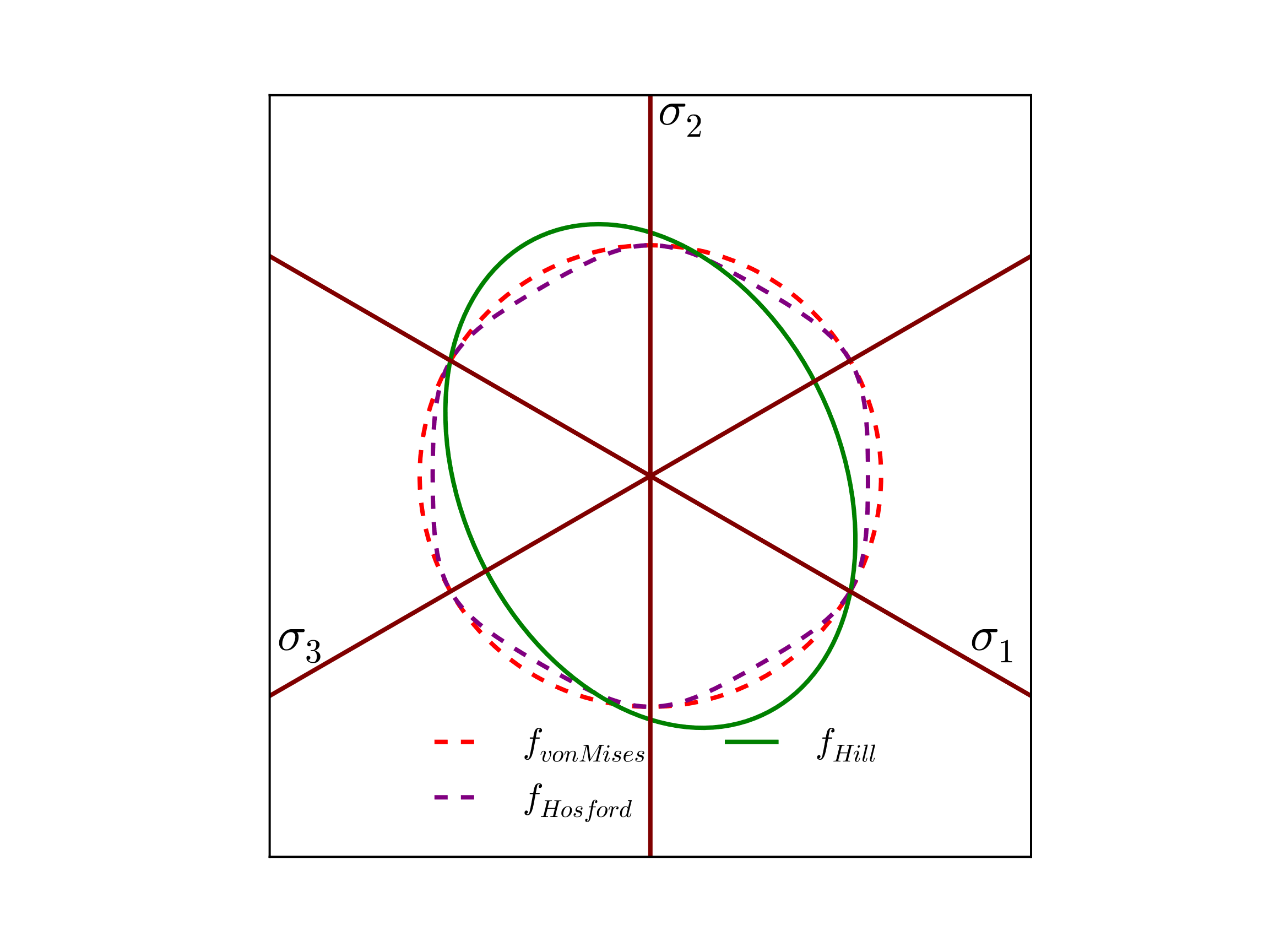
Fig. 4.58 Example anisotropic Hill yield surface, \(f_{Hill}\left(\sigma_{ij},\bar{\varepsilon}^p=0\right)\), presented in the deviatoric \(\pi\)-plane fit to 2090-T3 aluminum. Comparison von Mises (\(J_2\)) and Hosford (with \(a=8\)) surfaces are also presented.

The coefficients \(F\), \(G\), \(H\), \(L\), \(M\), and \(N\) were introduced by Hill. In terms of the yield stresses they are:

\[F = \frac{\left(\bar{\sigma}\right)^{2}}{2}\left[ \frac{1}{\left( \sigma_{22}^{y} \right)^{2}} + \frac{1}{\left( \sigma_{33}^{y} \right)^{2}} - \frac{1}{\left( \sigma_{11}^{y} \right)^{2}}\right] \;\;\; ; \;\;\; L = \frac{\left(\bar{\sigma}\right)^{2}}{2} \left[ \frac{1}{\left(\tau_{23}^{y}\right)^{2}} \right]\]

(4.48)\[G = \frac{\left(\bar{\sigma}\right)^{2}}{2}\left[ \frac{1}{\left( \sigma_{33}^{y} \right)^{2}} + \frac{1}{\left( \sigma_{11}^{y} \right)^{2}} - \frac{1}{\left( \sigma_{22}^{y} \right)^{2}} \right] \;\;\; ; \;\;\; M = \frac{\left(\bar{\sigma}\right)^{2}}{2} \left[ \frac{1}{\left(\tau_{31}^{y}\right)^{2}} \right]\]

\[H = \frac{\left(\bar{\sigma}\right)^{2}}{2}\left[ \frac{1}{\left( \sigma_{11}^{y} \right)^{2}} + \frac{1}{\left( \sigma_{22}^{y} \right)^{2}} - \frac{1}{\left( \sigma_{33}^{y} \right)^{2}} \right] \;\;\; ; \;\;\; N = \frac{\left(\bar{\sigma}\right)^{2}}{2} \left[ \frac{1}{\left(\tau_{12}^{y}\right)^{2}} \right].\]

where \(\bar{\sigma}\) is a reference yield stress.

Rather than input the six independent yield stresses, the ratios of the yield stresses to some reference yield stress are generally used as input. These ratios are

\[R_{11} = \frac{\sigma^{y}_{11}}{\bar{\sigma}} \;\;\; ; \;\;\; R_{12} = \sqrt{3}\frac{\tau^{y}_{12}}{\bar{\sigma}}\]

(4.49)\[R_{22} = \frac{\sigma^{y}_{22}}{\bar{\sigma}} \;\;\; ; \;\;\; R_{23} = \sqrt{3}\frac{\tau^{y}_{23}}{\bar{\sigma}}\]

\[R_{33} = \frac{\sigma^{y}_{33}}{\bar{\sigma}} \;\;\; ; \;\;\; R_{31} = \sqrt{3}\frac{\tau^{y}_{31}}{\bar{\sigma}}.\]

These ratios are set up so that if \(R_{ij} = 1\) then the yield surface is isotropic.

The orientation of the principal material axes with respect to the global Cartesian axes may be specified by the user. First, a rectangular or cylindrical reference coordinate system is defined. Spherical coordinate systems are not currently implemented for the Hill model. The material coordinate system can then be defined through two successive rotations about axes in the reference rectangular or cylindrical coordinate system. In the case of the cylindrical coordinate system this allows the principal material axes to vary point-wise in a given element block.

The plastic rate of deformation, as with the isotropic models, assumes associated flow

\[D_{ij}^{\text{p}} = \dot{\gamma} \frac{\partial\phi}{\partial\sigma_{ij}}.\]

Given the form for \(\phi\), the consistency parameter, \(\dot\gamma\) is equal to the rate of the equivalent plastic strain, \(\dot{\bar{\varepsilon}}^{p}\).

For more information about the Hill plasticity model, consult [[2]]. Additional discussion on options for failure models and adiabatic heating may be found in [[3], [4]] and [[5]], respectively.

4.15.1.1. Plastic Hardening

Plastic hardening refers to increases in the flow stress, \(\bar{\sigma}\), with plastic deformation. As such, hardening is described via a functional relationship between the flow stress and isotropic hardening variable (effective plastic strain), \(\bar{\sigma}\left(\bar{\varepsilon}^p\right)\). Over the course of nearly a century of work in metal plasticity, a variety of relationships have been proposed to describe the interactions associated with different physical interpretations, deformation mechanisms, and materials. To enable the utilization of the same plasticity models for different material systems, a modular implementation of plastic hardening has been adopted such that the analyst may select different hardening models from the input deck thereby avoiding any code changes or user subroutines. In this section, additional details are given for the different models to enable the user to select the appropriate choice of model. Note, the models being discussed here are only for isotropic hardening in which the yield surface expands. Kinematic hardening in which the yield surface translates in stress-space with deformation and distortional hardening where the shape of the yield surface changes shape with deformation are not treated. For a larger discussion of the phenomenology and history of different hardening types, the reader is referred to [[2], [6], [7]].

Given the ubiquitous nature of these hardening laws in computational plasticity, some (if not most) of this material may be found elsewhere in this manual. Nonetheless, the discussion is repeated here for the convenience of the reader.

4.15.1.1.1. Linear

Linear hardening is conceptually the simplest model available in LAMÉ. As the name implies, a linear relationship is assumed between the hardening variable, \(\bar{\varepsilon}^p\), and flow stress. The hardening modulus, \(H^{\prime}\), is a constant giving the rate of change of flow stress with plastic flow. The flow stress expression may therefore be written,

\[\bar{\sigma}=\sigma_y + H^{\prime}\bar{\varepsilon}^p.\]

The simplicity of the model is its main feature as the constant slope,

\[\frac{d\bar{\sigma}}{d\bar{\varepsilon}^p}=H^{\prime},\]

makes the model attractive for analytical models and cheap for computational implementations (e.g. radial return algorithms require only a single correction step). Unfortunately, the simplicity of the representation also means that it has limited predictive capabilities and can lead to overly stiff responses.

4.15.1.1.2. Power Law

Another common expression for isotropic hardening is the power-law hardening model. Due to its prevalence, a dedicated ELASTIC-PLASTIC POWER LAW HARDENING model may be found in LAMÉ (see Section 4.8.1). This expression is given as,

\[\bar{\sigma}=\sigma_y + A<\bar{\varepsilon}^p-\varepsilon_L>^n,\]

in which \(<\cdot>\) are Macaulay brackets, \(\varepsilon_L\) is the Luders strain, \(A\) is a fitting constant, and \(n\) is an exponent typically taken such that \(0<n\leq1\). The Luders strain is a positive, constant strain value (defaulted to zero) giving an initially perfectly plastic response in the plastic deformation domain (see Fig. 4.20). The derivative is then simply,

\[\frac{d\bar{\sigma}}{d\bar{\varepsilon}^p}=nA<\bar{\varepsilon}^p-\varepsilon_L>^{\left(n-1\right)}.\]

Note, one difficulty in such an implementation is that when the effective equivalent plastic strain is zero, numerical difficulties may arise in evaluating the derivative and necessitate special treatment of the case.

4.15.1.1.3. Voce

The Voce hardening model (sometimes referred to as a saturation model) uses a decaying exponential function of the equivalent plastic strain such that the hardening eventually saturates to a specified value (thus the name). Such a relationship has been observed in some structural metals giving rise to the popularity of the model. The hardening response is given as,

\[\bar{\sigma}=\sigma_y + A\left(1-\exp\left(-n\bar{\varepsilon}^p\right)\right),\]

in which \(A\) is a fitting constant and \(n\) is a fitting exponent controlling how quickly the hardening saturates. Importantly, the derivative is written as,

\[\frac{d\bar{\sigma}}{d\bar{\varepsilon}^p}=nA\exp\left(-n\bar{\varepsilon}^p\right),\]

and is well defined everywhere giving the selected form an advantage over the aforementioned power law model.

4.15.1.1.4. Johnson-Cook

The Johnson-Cook hardening model is a variant of the classical Johnson-Cook [[8], [9]] expression. In this instance, the temperature-dependence is neglected to focus on the rate-dependent capabilities while allowing for arbitrary isotropic hardening forms via the use of a user-defined hardening function. With these assumptions, the flow stress may be written as,

\[\bar{\sigma}=\tilde{\sigma}_y\left(\bar{\varepsilon}^p\right)\left[1+C\left<\ln\left(\frac{\dot{\bar{\varepsilon}}^p}{\dot{\varepsilon}_0}\right)\right>\right],\]

in which \(\tilde{\sigma}_y\left(\bar{\varepsilon}^p\right)\) is the user-specified rate-independent hardening function, \(C\) is a fitting constant and \(\dot{\varepsilon}_0\) is a reference strain rate. The Macaulay brackets ensure the material behaves in a rate independent fashion when \(\dot{\bar{\varepsilon}}^p < \dot{\varepsilon}_0\).

4.15.1.1.5. Power Law Breakdown

Like the Johnson-Cook formulation, the power-law breakdown model is also rate-dependent. Again, a multiplicative decomposition is assumed between isotropic hardening and the corresponding rate-dependence dependent. In this case, however, the functional form is derived from the analysis of Frost and Ashby [[10]] in which power-law relationships like those of the Johnson-Cook model cease to appropriately capture the physical response. The form used here is similar to the expression used by Brown and Bammann [[11]] and is written as,

\[\bar{\sigma} = \tilde{\sigma}_y\left(\bar{\varepsilon}^p\right)\left[1+\text{asinh}\left(\left(\frac{\dot{\bar{\varepsilon}}^p}{g}\right)^{\left(1/m\right)}\right)\right],\]

with \(\tilde{\sigma}_y\left(\bar{\varepsilon}^p\right)\) being the user supplied rate independent expression, \(g\) is a model parameter related to the activation energy required to transition from climb to glide-controlled deformation, and \(m\) dictates the strength of the dependence.

4.15.1.2. Flow Stress

Unlike the previously described models, the flow-stress hardening method is less a specific physical representation and more a generalization of hardening behaviors to allow greater flexibility in separately describing isotropic hardening, rate-dependence, and temperature dependence. As such, the generic flow-stress definition of

\[\bar{\sigma}\left(\bar{\varepsilon}^p,\dot{\bar{\varepsilon}}^p,\theta\right)=\tilde{\sigma}_y\left(\bar{\varepsilon}^p\right)\hat{\sigma}\left(\dot{\bar{\varepsilon}}^p\right)\breve{\sigma}\left(\theta\right),\]

is used in which \(\hat{\sigma}\) and \(\breve{\sigma}\) are rate and temperature multipliers, respectively, that by default are unity (such that the response is rate and temperature independent). The isotropic hardening component, \(\tilde{\sigma}_y\), is specified as,

\[\tilde{\sigma}_y=\sigma_y+K\left(\bar{\varepsilon}^p\right),\]

with \(\sigma_y\) being the constant yield stress and \(K\) is the isotropic hardening that is initially zero and a function of the equivalent plastic strain. A multiplicative decomposition such as this mirrors the general structure used by Johnson and Cook [[8], [9]] although greater flexibility is allowed in terms of the specific form of the rate and temperature multipliers.

Given the aforementioned defaults for rate and temperature dependence, the corresponding multipliers need not be specified. A representation for the isotropic hardening, however, must be specified and can be defined via linear, power-law, Voce, or user-defined representations. For the user-defined case, an isotropic hardening function is required and it must be highlighted that the interpretation differs from the general user-defined hardening model. In this case, as the specified function represents the isotropic hardening, it should start from zero – not yield.

Although the flow-stress hardening model defaults to rate and temperature independent, a multiplier may be defined for either (or both) of the terms. For rate-dependence, either the previously discussed Johnson-Cook or power-law breakdown models or a user-defined multiplier may be used. For the user-defined capability, the multiplier should be input as a strictly positive function of the equivalent plastic strain rate with a value of one in the rate-independent limit.

In terms of temperature dependence, the multiplier may be specified given a Johnson-Cook dependency [[8], [9]],

\[\breve{\sigma}\left(\theta\right)=1-\left(\frac{\theta-\theta_{\text{ref}}}{\theta_{\text{melt}}-\theta_{\text{ref}}}\right)^M,\]

with \(\theta_{\text{ref}},~\theta_{\text{melt}}\) and \(M\) being the reference temperature, melting temperature, and temperature exponent. The temperature multiplier may also be specified via a user defined function.

4.15.1.3. Decoupled Flow Stress

Like the flow-stress hardening method, the decoupled flow-stress hardening implementation is a generalization of the hardening behaviors to allow greater flexibility. In differentiating the two, for the decoupled model the rate and temperature dependence may be separately specified for the yield and hardening portions of the flow stress. As such, the generic flow-stress definition of

\[\bar{\sigma}\left(\bar{\varepsilon}^p,\dot{\bar{\varepsilon}}^p,\theta\right)=\sigma_y\hat{\sigma}_{\text{y}}\left(\dot{\bar{\varepsilon}}^p\right)\breve{\sigma}_{\text{y}}\left(\theta\right)+K\left(\bar{\varepsilon}^p\right)\hat{\sigma}_{\text{h}}\left(\dot{\bar{\varepsilon}}^p\right)\breve{\sigma}_{\text{h}}\left(\theta\right),\]

is used in which \(\hat{\sigma}\) and \(\breve{\sigma}\) are rate and temperature multipliers, respectively, that by default are unity (such that the response is rate and temperature independent) with subscripts y and h denoting functions associated with yield and hardening. The isotropic hardening is described by \(K\left(\bar{\varepsilon}^p\right)\) and \(\sigma_y\) is the constant initial yield stress. It may also be seen that if the yield and hardening dependencies are the same (\(\hat{\sigma}_{\text{y}}=\hat{\sigma}_{\text{h}}\) and \(\breve{\sigma}_{\text{y}}=\breve{\sigma}_{\text{h}}\)) the decoupled flow stress model reduces to that of the flow stress case and mirrors the general structure of the Johnson-Cook model [[8], [9]].

Given the aforementioned defaults for rate and temperature dependence, the corresponding multipliers need not be specified. A representation for the isotropic hardening, however, must be specified and can be defined via linear, power-law, Voce, or user-defined representations. For the user-defined case, an isotropic hardening function should be used and it must be highlighted that the interpretation differs from the general user-defined hardening model. In this case, as the specified function represents the isotropic hardening, it should start from zero – not yield.

Although the decoupled flow-stress hardening model defaults to rate and temperature independent, a multiplier may be defined for any of the terms. For rate-dependence, either the previously discussed Johnson-Cook or power-law breakdown models or a user-defined multiplier may be used. For the user-defined capability, the multiplier should be input as a strictly positive function of the equivalent plastic strain rate with a value of one in the rate-independent limit.

In terms of temperature dependence, the multiplier may be specified given a Johnson-Cook dependency [[8], [9]],

\[\breve{\sigma}\left(\theta\right)=1-\left(\frac{\theta-\theta_{\text{ref}}}{\theta_{\text{melt}}-\theta_{\text{ref}}}\right)^M,\]

where \(\theta_{\text{ref}},~\theta_{\text{melt}}\), and \(M\) are the reference temperature, melting temperature, and temperature exponent. A temperature multiplier may also be specified via a user defined function.

4.15.2. Implementation

The Hill plasticity model uses a predictor-corrector algorithm for integrating the constitutive model. Given a rate of deformation, ifindex \(d_{ij}\)else \({\bf d}\)fi, and a time step, \(\Delta\,t\), a trial stress state is calculated based on an elastic response

\[T_{ij}^{tr} = T_{ij}^{n} + \Delta\,t \, \mathbb{C}_{ijkl}d_{kl}\]

If the trial stress state lies outside the yield surface, i.e. if ifindex \(\phi(T_{ij}^{tr}) > \bar{\sigma}\)else \(\phi({\bf T}^{tr}) > \bar{\sigma}\)fi, then the model uses a backward Euler algorithm to return the stress to the yield surface. There are two equations that need to be solved. To ensure that the plastic strain increment is in the correct direction we have

\[R^{p}_{ij} = \Delta t \, d_{ij}^{p} - \Delta\gamma \frac{\partial\phi}{\partial T_{ij}} = 0\]

while to ensure that the stress state is on the yield surface we require

\[f = \phi\left( T_{ij} \right) - \bar{\sigma}\left( \bar{\varepsilon}^{p} \right) = 0\]

The primary algorithm for solving these equations is a Newton-Raphson algorithm. Using \(\Delta \gamma\) (which is equal to \(\Delta\bar{\varepsilon}^{p}\)) and ifindex \(T_{ij}\)else \({\bf T}\)fi as the solution variables, we set up an iterative algorithm where

\[\begin{split}\Delta \gamma^{(k+1)} & = \Delta \gamma^{(k)} + \Delta\left(\Delta\gamma\right) \nonumber \\ \\ T_{ij}^{(k+1)} & = T_{ij}^{(k)} + \Delta T_{ij} \nonumber\end{split}\]

where \(\Delta\gamma^{(0)} = 0\) and ifindex \(T_{ij}^{(0)} = T_{ij}^{tr}\)else \({\bf T}^{(0)} = {\bf T}^{tr}\)fi and

\[\Delta t \, d_{ij}^{p} = \mathbb{C}^{-1}_{ijkl} \left( T_{kl}^{tr} - T_{kl} \right)\]

The Newton-Raphson algorithm gives

\[\begin{split}\Delta\left( \Delta \gamma \right) & = \frac{\displaystyle f^{(k)} - R_{ij}^{(k)} \, \mathcal{L}^{(k)}_{ijkl} \, \frac{\partial\phi^{(k)}}{\partial T_{kl}}} {\displaystyle \frac{\partial\phi^{(k)}}{\partial T_{ij}} \, \mathcal{L}^{(k)}_{ijkl} \, \frac{\partial\phi^{(k)}}{\partial T_{kl}} + H^{\prime \, (k)}} \nonumber \\ \\ \Delta T_{ij} & = - \mathcal{L}^{(k)}_{ijkl} \, \left( R_{kl}^{(k)} + \Delta\left(\Delta\gamma\right)\frac{\partial\phi^{(k)}}{\partial T_{kl}}\right) \nonumber\end{split}\]

A straightforward Newton-Raphson algorithm does not always converge, so the return mapping algorithm is augmented with a line search algorithm

\[\begin{split}\Delta \gamma^{(k+1)} & = \Delta \gamma^{(k)} + \alpha \Delta\left(\Delta\gamma\right) \nonumber \\ \\ T_{ij}^{(k+1)} & = T_{ij}^{(k)} + \alpha \Delta T_{ij} \nonumber\end{split}\]

where \(\alpha \in (0,1]\) is the line search parameter which is determined from certain convergence considerations. If \(\alpha = 1\) then the Newton-Raphson algorithm is recovered. The line search algorithm greatly increases the reliability of the return mapping algorithm.

4.15.3. Verification

The Hill plasticity material model is verified for a number of loading conditions.

Additional verification exercises for the various failure models and adiabatic heating capabilities may be found in [[3], [4]] and [[5]], respectively.

The elastic properties used in these analyses are \(E = 70\) GPa and \(\nu = 0.25\). The parameters that are used to define the yield surface are

\[\begin{split}R_{11} = 1.000680 \;\;\; ; \;\;\; R_{12} = 0.909194 \nonumber \\ \nonumber \\ R_{22} = 0.906397 \;\;\; ; \;\;\; R_{23} = 0.851434 \\ \nonumber \\ R_{33} = 1.027380 \;\;\; ; \;\;\; R_{31} = 0.799066\end{split}\]

These parameters correspond to a parameterization of the Barlat model for 2090-T3 aluminum [[12]] that is fit to the Hill model. The hardening law used for the model is a Voce law with the following form

\[\bar{\sigma}\left(\bar{\varepsilon}^{p}\right) = \sigma_{y} + A \left( 1 - \exp(-n \bar{\varepsilon}^{p})\right)\]

For these calculations \(\sigma_{y} = 200\) MPa, \(A = 200\) MPa, and \(n = 20\). Finally, the coordinate system used in these calculations is a rectangular coordinate system with the \(e_{1},e_{2},e_{3}\) axes aligned with the \(x,y,z\) axes.

4.15.3.1. Uniaxial Stress

The Hill plasticity model is tested in uniaxial tension along the three orthogonal principal material directions. The tests looks at the stress, the strain, and the equivalent plastic strain and compares these values against analytical results for the same problem. In this verification problem only the normal stresses are needed, and the shear terms are not exercised. Therefore, the parameters \(R_{12}\), \(R_{23}\), and \(R_{31}\) are not used in the problem and a separate verification test will be needed for shear response.

The model is tested in uniaxial stress in the \(x\), \(y\), and \(z\) directions, giving three test problems. Each problem can be formulated exactly the same. For the description of the test we will only look at loading in the \(x\) direction (\(x_{1}\) direction).

For the uniaxial stress problem, the only non-zero stress component is \(\sigma_{11}\). In the analysis that follows \(\sigma_{11} = \sigma\). There are three non-zero strain components, \(\varepsilon_{11}\), \(\varepsilon_{22}\), and \(\varepsilon_{33}\). In the analysis that follows \(\varepsilon_{11} = \varepsilon\). Furthermore, the axial elastic strain, \(\varepsilon_{11}^{\text{e}} = \sigma/E\) will be denoted by \(\varepsilon^{\text{e}}\).

4.15.3.1.1. Axial Stresses

The uniaxial stress calculated by the model in Adagio is compared to analytical solutions. For uniaxial loading in the \(e_{1}\) direction, the effective stress is

\[\phi = \frac{\sigma}{R_{11}}\]

If the stress state is on the yield surface, then \(\phi = \bar{\sigma}\left(\bar{\varepsilon}^{p}\right)\), so the axial stress, as a function of the hardening function, is

(4.50)\[\sigma = R_{kk}\bar{\sigma}\left(\bar{\varepsilon}^{p}\right)\]

This shows that the stress state can be calculated from the hardening law and the anisotropy parameters.

To evaluate the axial stress we need the equivalent plastic strain as a function of the axial strain. If we equate the rate of plastic work we get

\[\bar{\sigma} \dot{\bar{\varepsilon}}^{p} = \sigma \left( \dot\varepsilon - \dot\varepsilon^{\text{e}} \right) \;\;\; \rightarrow \;\;\; \dot{\bar{\varepsilon}}^{p} = R_{11} \left( \dot\varepsilon - \dot\varepsilon^{\text{e}} \right)\]

which, when integrated, gives us an implicit equation for the equivalent plastic strain

(4.51)\[\bar{\varepsilon}^{p} = R_{11} \left( \varepsilon - R_{11} \frac{\bar{\sigma}(\bar{\varepsilon}^{p})}{E} \right)\]

The equivalent plastic strain can then be used in (4.50) to find the axial stress, \(\sigma\).

The axial stresses for loading in the other directions can be found the same way. The axial stresses for loading in the \(e_{1}\), \(e_{2}\), and \(e_{3}\) directions are shown in Fig. 4.59.

4.15.3.1.2. Lateral Strains

For the lateral strains we need the plastic strains and therefore the normal to the yield surface. The components of the normal to the yield surface are

\[\frac{\partial\phi}{\partial \sigma_{11}} = \frac{1}{R_{11}} \;\;\; ; \;\;\; \frac{\partial\phi}{\partial \sigma_{22}} = - H R_{11} \;\;\; ; \;\;\; \frac{\partial\phi}{\partial \sigma_{33}} = - G R_{11}\]

The elastic axial and lateral strain components are

\[\varepsilon^{\text{e}}_{11} = \frac{\sigma}{E} = \varepsilon^{\text{e}} \;\;\; ; \;\;\; \varepsilon^{\text{e}}_{22} = \varepsilon^{\text{e}}_{33} = -\nu\frac{\sigma}{E} = -\nu\varepsilon^{\text{e}}\]

The plastic axial strain component is

\[\varepsilon^{\text{p}}_{11} = \varepsilon_{11} - \frac{\sigma}{E} = \varepsilon - \varepsilon^{\text{e}}\]

which comes from the additive decomposition of the strain rates. Using the equivalent plastic strain~:eq:eq:verhilleqps we can find the lateral plastic strain components

\[\varepsilon^{\text{p}}_{22} = - \left( \varepsilon - \varepsilon^{\text{e}} \right) H R_{11}^{2} \;\;\; ; \;\;\; \varepsilon^{\text{p}}_{33} = - \left( \varepsilon - \varepsilon^{\text{e}} \right) G R_{11}^{2}\]

The lateral total stain components prior to yield are \(\varepsilon_{22} = \varepsilon_{33} = -\nu \varepsilon\). After yield they are

\[\begin{split}\varepsilon_{22} & = -\nu \varepsilon^{\text{e}} - H R_{11} \bar{\varepsilon}^{p} \nonumber \\ \\ \varepsilon_{33} & = -\nu \varepsilon^{\text{e}} - G R_{11} \bar{\varepsilon}^{p} \nonumber\end{split}\]

where \(\varepsilon^{\text{e}} = \sigma/E\).

For loading in the \(y\) direction, a similar analysis leads to the lateral strains, after yield

\[\begin{split}\varepsilon_{33} & = -\nu \varepsilon^{\text{e}} - F R_{22} \bar{\varepsilon}^{p} \nonumber \\ \\ \varepsilon_{11} & = -\nu \varepsilon^{\text{e}} - H R_{22} \bar{\varepsilon}^{p} \nonumber\end{split}\]

For loading in the \(z\) direction, a similar analysis leads to the lateral strains, after yield

\[\begin{split}\varepsilon_{11} & = -\nu \varepsilon^{\text{e}} - G R_{33} \bar{\varepsilon}^{p} \nonumber \\ \\ \varepsilon_{22} & = -\nu \varepsilon^{\text{e}} - F R_{33} \bar{\varepsilon}^{p} \nonumber\end{split}\]

Results for all three loadings are shown in Fig. 4.60, Fig. 4.61, and Fig. 4.62.

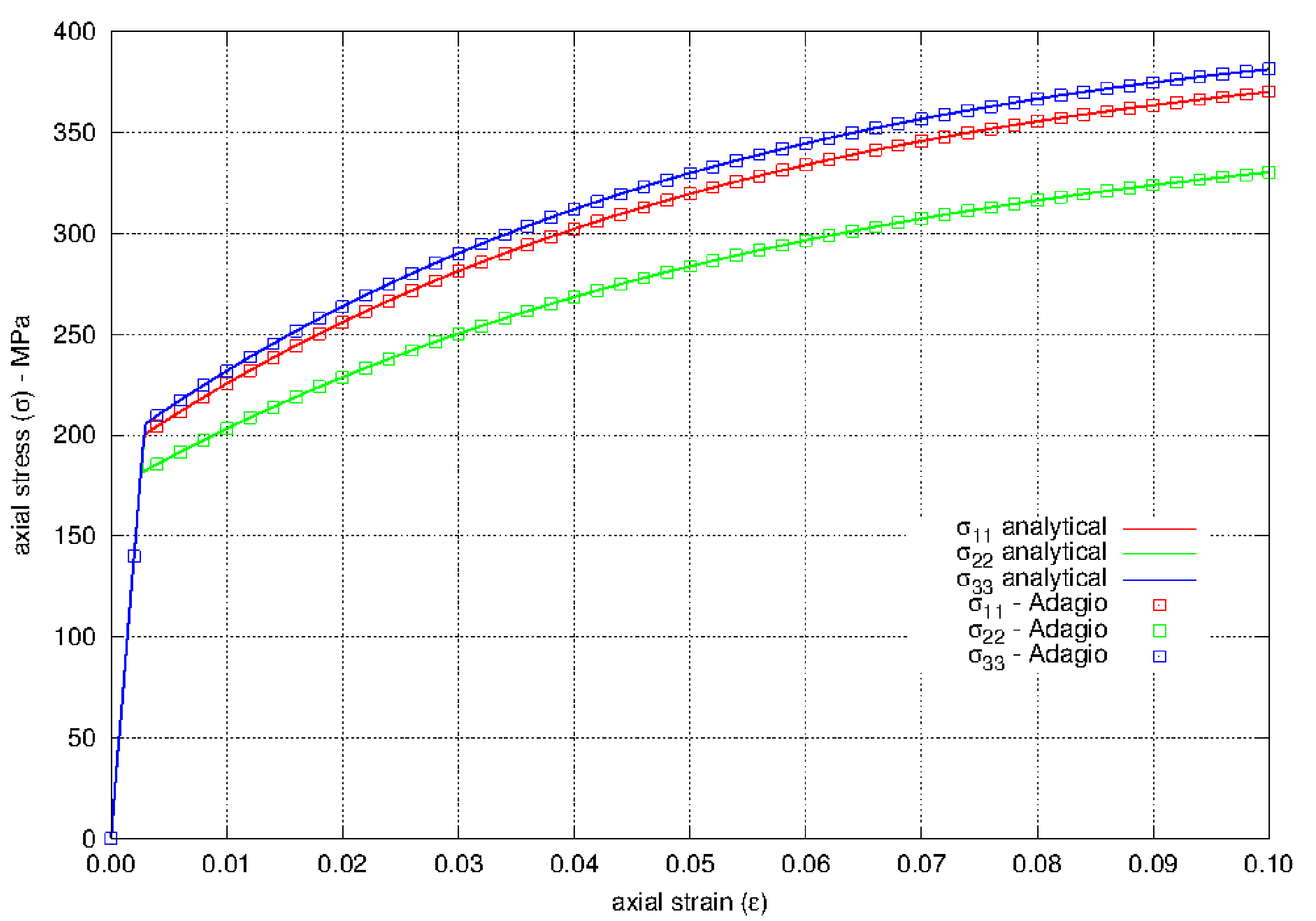
Fig. 4.59 Stresses when loading in the \(e_{1}\), \(e_{2}\), and \(e_{3}\)-directions using the Hill model with a Voce hardening law.

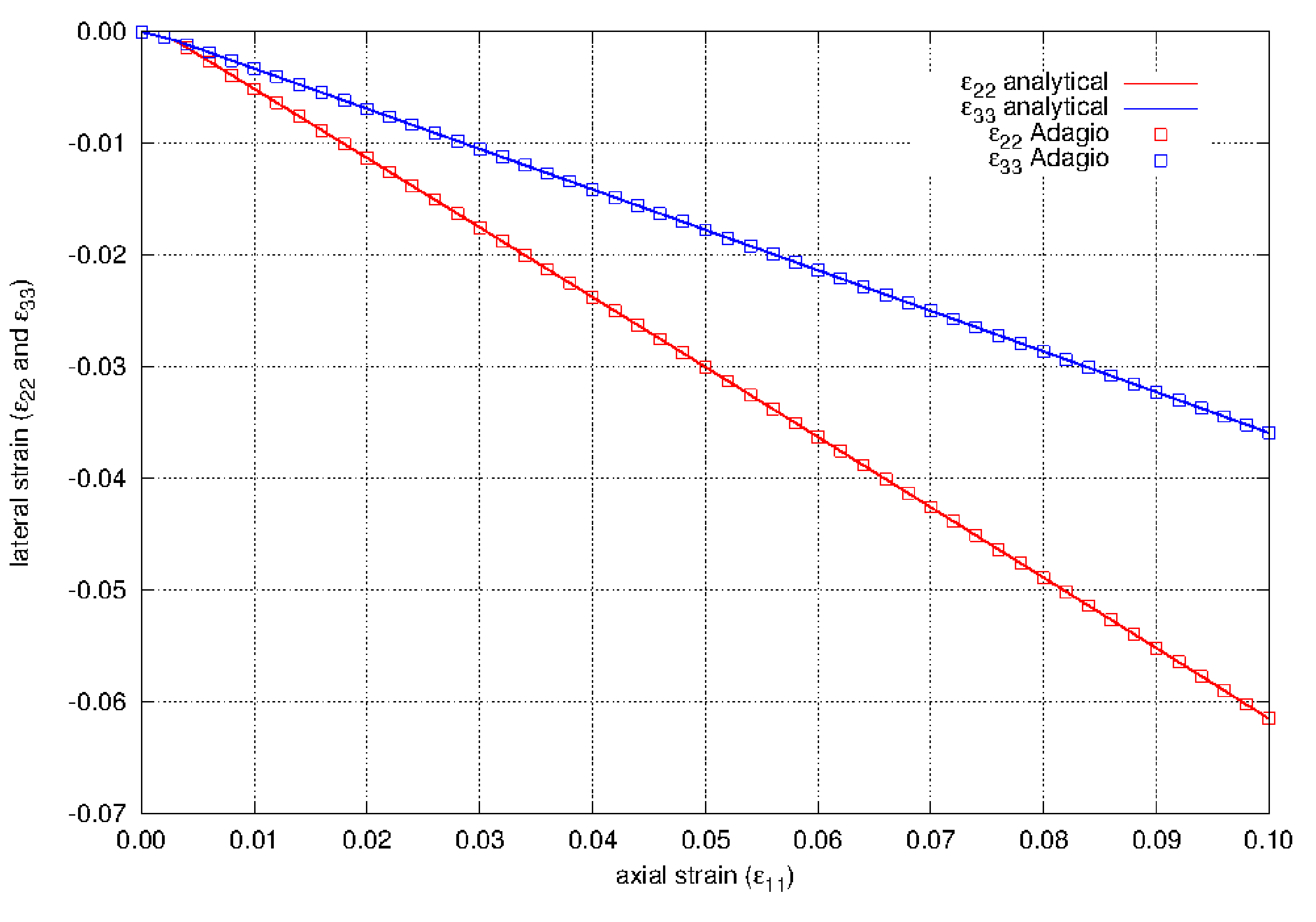
Fig. 4.60 Lateral strain as a function of axial strain for the Hill model of 2090-T3 aluminum. Loading is in the \(e_{1}\)-direction and the hardening law is a Voce law.

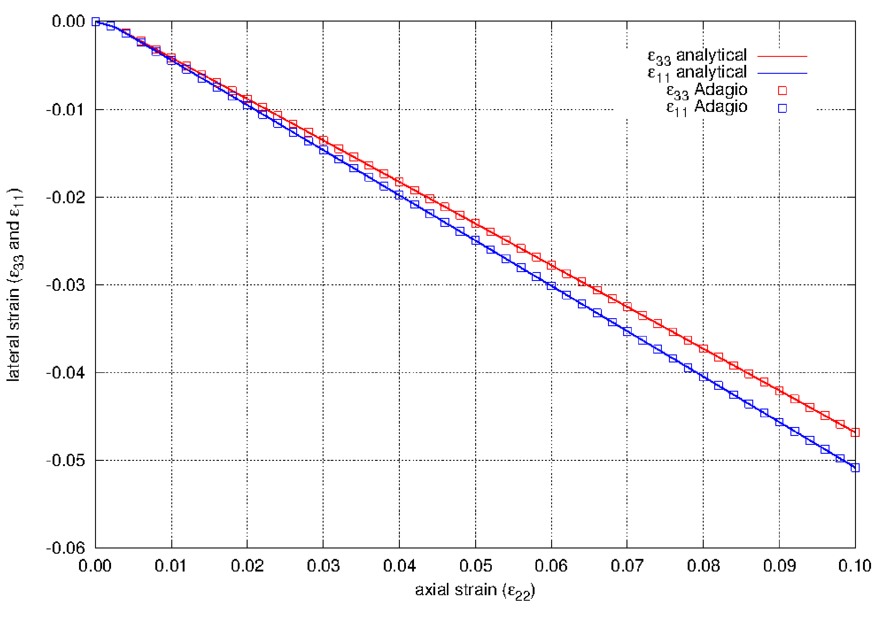
Fig. 4.61 Lateral strain as a function of axial strain for the Hill model of 2090-T3 aluminum. Loading is in the \(e_{2}\)-direction and the hardening law is a Voce law.

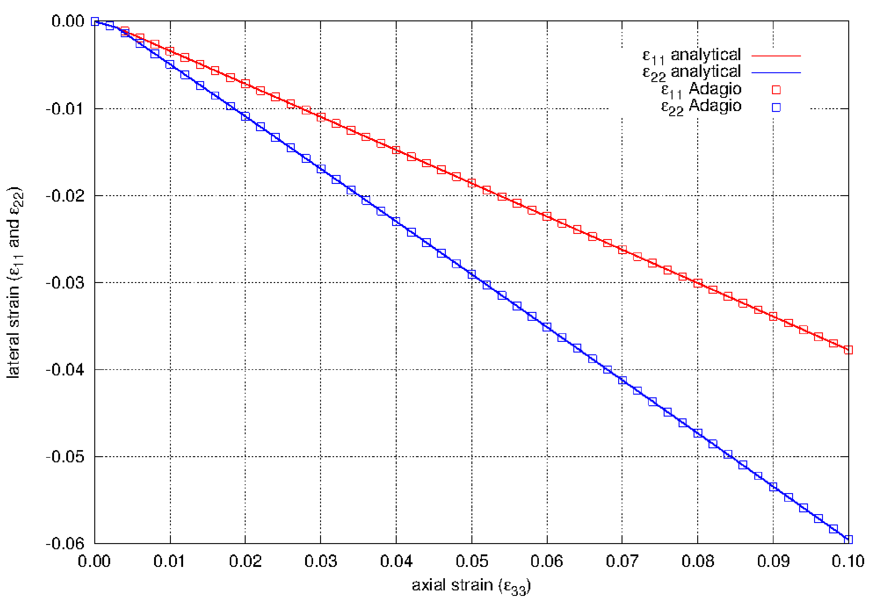
Fig. 4.62 Lateral strain as a function of axial strain for the Hill model of 2090-T3 aluminum. Loading is in the \(e_{3}\)-direction and the hardening law is a Voce law.

4.15.3.2. Pure Shear

The shear stress calculated by the Hill plasticity model in Adagio is compared to analytical solutions. Without loss of generality we will look at solutions for pure shear with respect to the \(e_{1}\)-\(e_{2}\) axes. Solutions for shear with respect to the other axes will be similar. In what follows, the only non-zero shear stress will be \(\sigma_{12}\), and the only non-zero shear strain will be \(\varepsilon_{12}\) In general, for pure shear with respect to the \(e_{1}\)-\(e_{2}\) axes, the effective stress is

\[\phi = \sqrt{3} \, \frac{\sigma_{12}}{R_{12}}\]

If the stress state is on the yield surface, then \(\phi = \bar{\sigma}\left(\bar{\varepsilon}^{p}\right)\), so the shear stress is

(4.52)\[\sigma_{12} = \frac{R_{12}}{\sqrt{3}}\bar{\sigma}\left(\bar{\varepsilon}^{p}\right)\]

This shows that the pure shear stress state can be calculated from the hardening law and the anisotropy parameters.

To evaluate the shear stress we need the equivalent plastic strain as a function of the shear strain. If we equate the rate of plastic work we get

\[\bar{\sigma}\dot{\bar{\varepsilon}}^{p} = 2 \sigma_{12} \left( \dot{\varepsilon}_{12} - \dot{\varepsilon}_{12}^{\text{e}} \right) \;\;\; \rightarrow \;\;\; \dot{\bar{\varepsilon}}^{p} = \frac{2 R_{12}}{\sqrt{3}} \left( \dot{\varepsilon}_{12} - \dot{\varepsilon}_{12}^{\text{e}} \right)\]

which, when integrated, gives us an implicit equation for the equivalent plastic strain

\[\bar{\varepsilon}^{p} = \frac{2 R_{12}}{\sqrt{3}} \left( \varepsilon_{12} - \frac{R_{12}}{\sqrt{3}} \frac{\bar{\sigma}\left(\bar{\varepsilon}^{p}\right)}{2\,G} \right)\]

If we define \(\hat{R}_{12} = R_{12}/\sqrt{3}\) then we get a form similar to what we had for uniaxial stress

\[\bar{\varepsilon}^{p} = 2 \hat{R}_{12} \left( \varepsilon_{12} - \hat{R}_{12} \frac{\bar{\sigma}\left(\bar{\varepsilon}^{p}\right)}{2\,G} \right)\]

The equivalent plastic strain can now be used to find the shear stress.

4.15.3.2.1. Boundary Conditions for Pure Shear

The deformation gradient that gives pure shear for loading relative to the \(e_{1}\)-\(e_{2}\) axes is

\[\begin{split}\left[ {\bf F} \right] = \begin{bmatrix} \frac{1}{2} \left( \lambda + \lambda^{-1} \right) & \frac{1}{2} \left( \lambda - \lambda^{-1} \right) & 0 \\ \\ \frac{1}{2} \left( \lambda - \lambda^{-1} \right) & \frac{1}{2} \left( \lambda + \lambda^{-1} \right) & 0 \\ \\ 0 & 0 & 1 \end{bmatrix} \;\;\; \rightarrow \;\;\; \left[ {\boldsymbol{\varepsilon}} \right] = \begin{bmatrix} 0 & \varepsilon & 0 \\ \\ \varepsilon & 0 & 0 \\ \\ 0 & 0 & 0 \end{bmatrix} \;\;\; ; \;\;\; \varepsilon = \ln\lambda\end{split}\]

For loading relative to the \(e_{2}\)-\(e_{3}\) axes and the \(e_{3}\)-\(e_{1}\) axes the boundary conditions are modified appropriately.

4.15.3.2.2. Results

The results for the Hill plasticity model loaded in pure shear are shown in Fig. 4.63. We see that the stress strain curves in pure shear as calculated by Adagio follow the expected stress strain curves. All other stress and strain components for the three problems are zero.

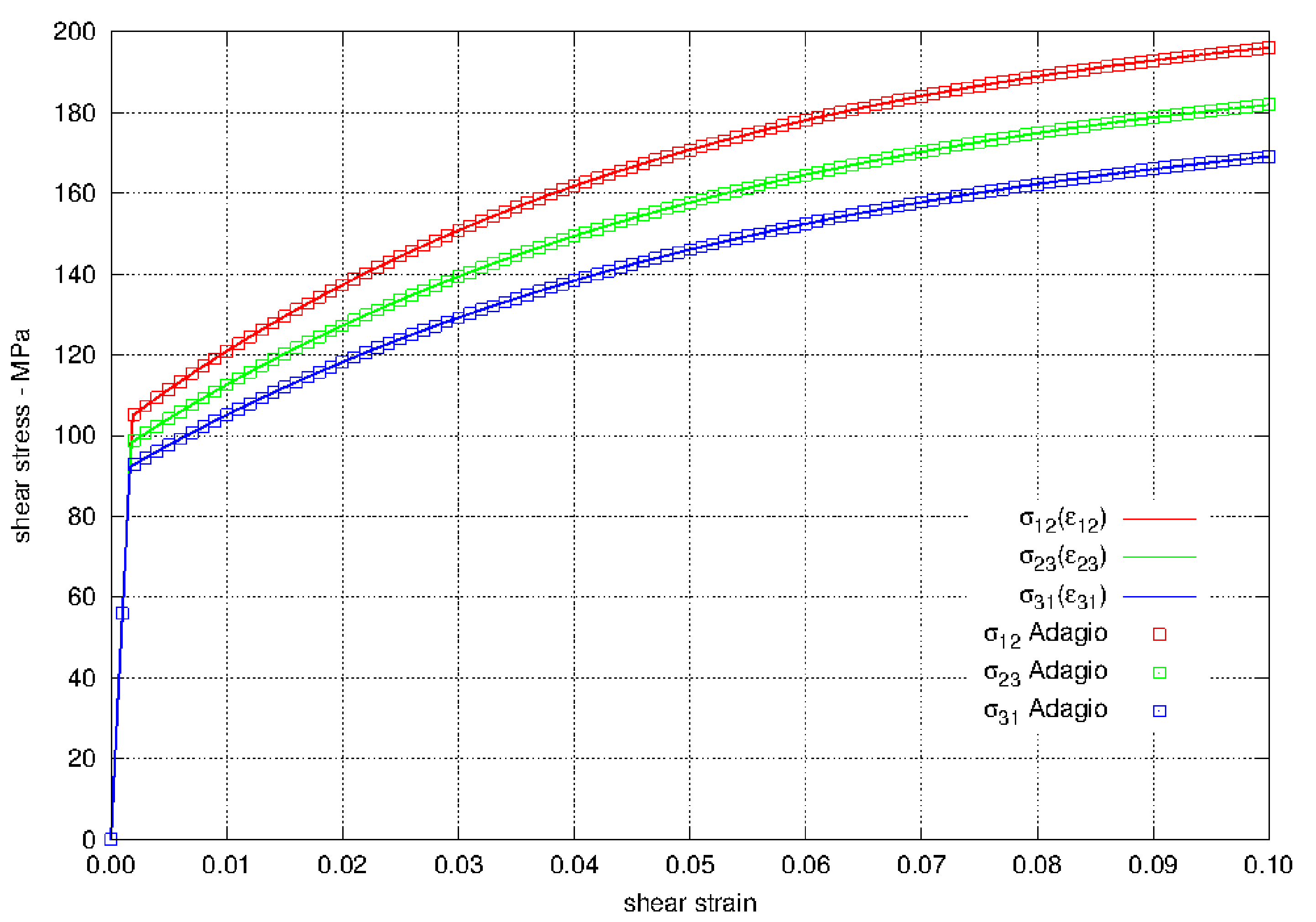
Fig. 4.63 Shear stress versus shear strain using the Hill model with a Voce hardening law. Results are for shear in the three orthogonal planes of the material coordinate system.

4.15.3.3. Plastic Hardening

To verify the capabilities of the hardening models, rate independent and rate dependent alike, the constant equivalent plastic strain rate, \(\dot{\bar{\varepsilon}}^p\), uniaxial stress and pure shear verification tests described in Appendix A are utilized. In these simplified loading cases, the material state may be found explicitly as a function of time knowing the prescribed equivalent strain rate. For the rate independent cases, a strain rate of \(\dot{\bar{\varepsilon}}^p=1\times10^{-4} \text{s}^{-1}\) is used for ease in simulations although the selected rate does not affect the results. Through this testing protocol, the hardening models are not only tested at different rates but also in different principal material directions to consider the anisotropy of the Hill yield surface. Additionally, the rate dependent models are tested for a wide range of strain rates (over five decades) and with all three rate independent hardening functions (\(\tilde{\sigma}_y\) in the previous theory section). Although linear, Voce, and power-law rate independent representations are utilized in the rate dependent tests, in those cases the hardening models are prescribed via user-defined analytic functions. The rate independent verification exercises, on the other hand, examine the built in hardening models. This distinction necessitates the different considerations and treatments.

The various rate dependent and rate independent hardening coefficients are found in Table 4.20 while the remaining model parameters are unchanged from the previous verification exercises. For the current verification exercises, the rate independent hardening models (linear, Voce, and power-law) will first be considered and then the rate dependent forms (Johnson-Cook, power-law breakdown).

Table 4.20 The model parameters for the hardening verification tests used with the Hill plasticity model during verification tests. Parameters for the rate independent hardening functions, \(\tilde{\sigma}_y\), are also given and denoted with a \(\tilde{\cdot}\) while the subscript refers to the functional form.

\(C\)	0.1	\(\dot{\varepsilon}_0\)	\(1\times 10^{-4}\) s\(^{-1}\)
\(g\)	0.21 s\(^{-1}\)	\(m\)	16.4
\(\tilde{H}_{\text{Linear}}\)	200 MPa
\(\tilde{A}_{\text{PL}}\)	400 MPa	\(\tilde{n}_{\text{PL}}\)	0.25
\(\tilde{A}_{\text{Voce}}\)	200 MPa	\(\tilde{n}_{\text{Voce}}\)	20

4.15.3.3.1. Linear

To examine the performance of the rate independent linear hardening model, the verification exercises from Appendix A are used. In this case, as the Hill yield surface is being considered, the responses are determined numerically and analytically in the uniaxial stress case with loading in three different principal material directions and three different shear planes for the pure shear case. These results are presented in Fig. 4.64. From these responses, superb agreement between the analytical and numerical results is noted. Additionally, the constant linear stress-strain response during plastic deformations clearly demonstrates the behavior giving this model its name.

Uniaxial Stress

Pure Shear

Fig. 4.64 Uniaxial stress-strain (a) and pure shear (b) responses of the Hill plasticity model with rate independent, linear hardening. Solid lines are analytical while open symbols are numerical.

4.15.3.3.2. Power-Law

The rate independent power-law hardening model is verified by using the uniaxial stress and pure shear problems of Appendix A. Results of these endeavors determined analytically and numerically are presented in Fig. 4.65 in which the uniaxial stress problem is presented for loading aligned with the three different principal material directions and three different shear planes for the pure shear case. From these results, outstanding agreement is noted between both numerical and analytical results sets verifying the model. Also, the initially stiff hardening decreasing to a lower linear tangent modulus characteristic of power-law hardening models is clearly evident in the various result sets of Fig. 4.65.

Uniaxial Stress

Pure Shear

Fig. 4.65 Uniaxial stress-strain (a) and pure shear (b) responses of the Hill plasticity model with rate independent, power-law hardening. Solid lines are analytical while open symbols are numerical.

4.15.3.3.3. Voce

Verification of the rate independent Voce hardening model is pursued by considering both the uniaxial stress and pure shear approaches of Appendix A. The results of these investigations determined analytically and numerically are shown in Fig. 4.66. For the uniaxial stress cases, loadings in each of the three principal material directions is presented while complementary results from the three shear planes are shown for the pure shear case. In each of these six instances, exemplary agreement is observed between the different results sets. Additionally, such stress-strain results also show the saturation behavior associated with Voce models in which at some equivalent plastic strain the material no longer hardens.

Uniaxial Stress

Pure Shear

Fig. 4.66 Uniaxial stress-strain (a) and pure shear (b) responses of the Hill plasticity model with rate independent, Voce hardening. Solid lines are analytical while open symbols are numerical.

4.15.3.3.4. Johnson-Cook

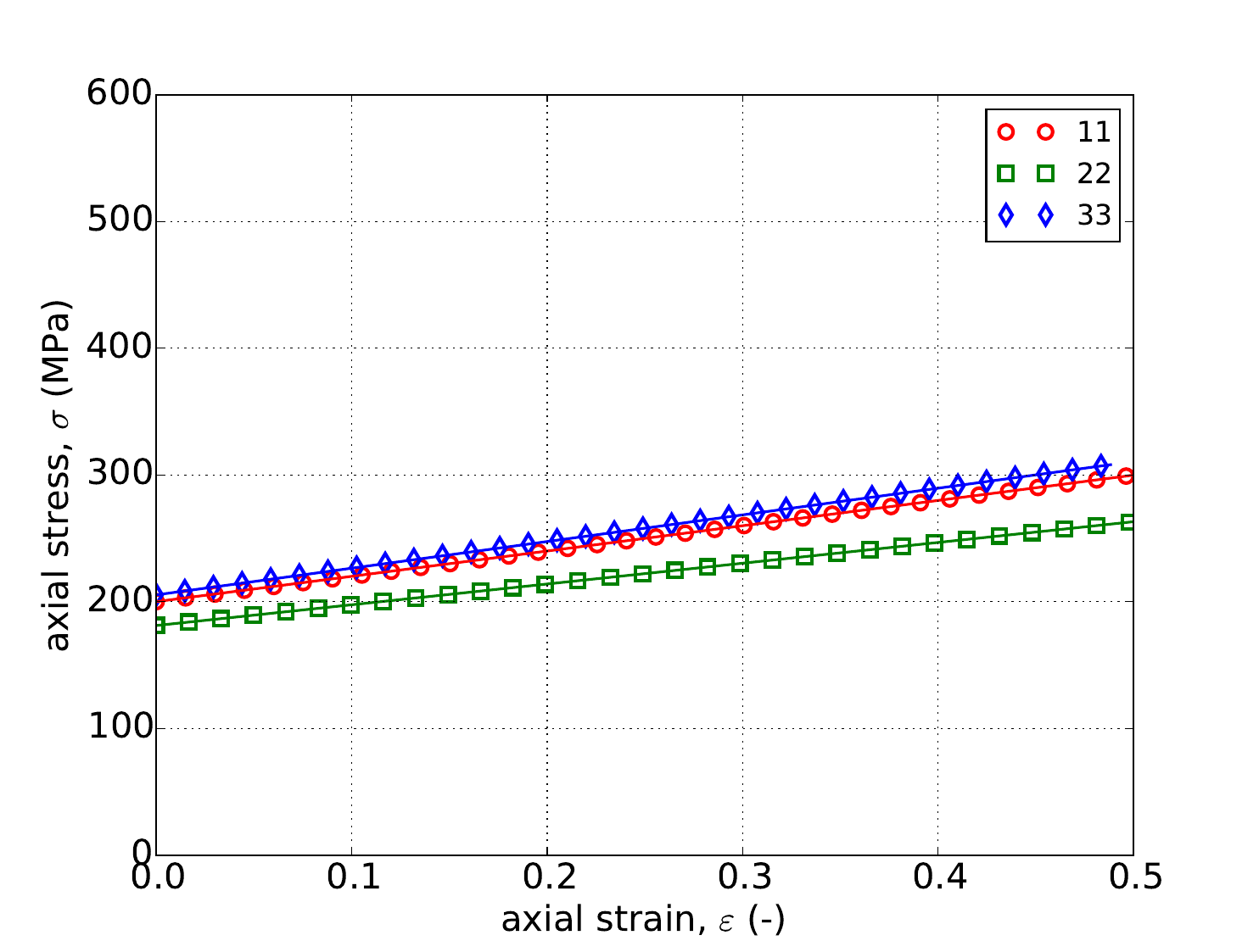
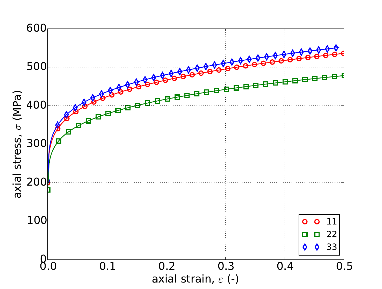
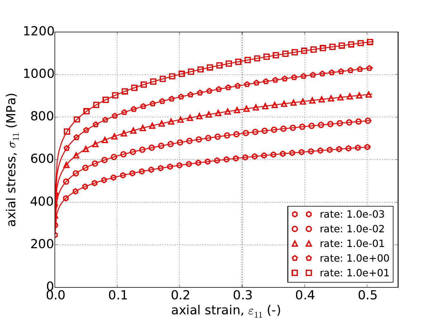
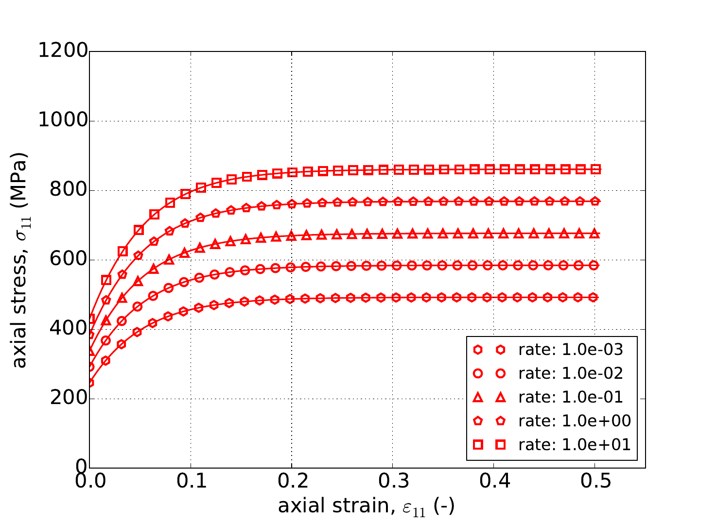
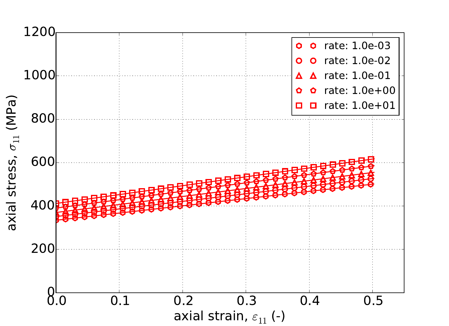
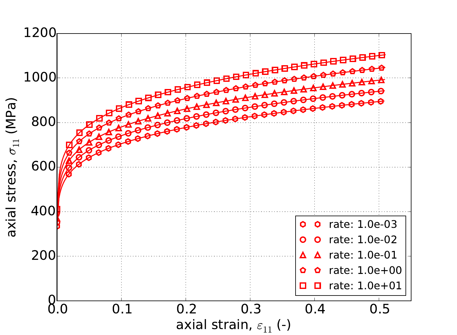
As noted in Appendix A, the uniaxial stress response depends on the yield surface anisotropy coefficients (for the Hill model the \(R's\)). The respective coefficients are given in the aforementioned appendix while Fig. 4.67 and Fig. 4.68 present the results of forty-five different verification exercises corresponding to different combinations of the three material principal directions (\(\hat{e}_1,~\hat{e}_2,\) and \(\hat{e}_3\)), five equivalent plastic strain rates(\(1\times10^{-3},~1\times10^{-2},~1\times10^{-1},~1\times10^{0}\) and \(1\times10^1~\text{s}^{-1}\)), and three rate independent hardening models (linear, power-law, and Voce). For each combination, the analytical and numerical results match to within acceptably small numerical differences.

Linear Hardening -- 11

Linear Hardening -- 22

Linear Hardening -- 33

Power-Law Hardening -- 11

Power-Law Hardening -- 22

Power-Law Hardening -- 33

Fig. 4.67 Uniaxial stress-strain response of the Hill plasticity model with rate dependent, Johnson-Cook type hardening with (a-c) linear and (d-f) power-law rate independent hardening. Solid lines are analytical results while open symbols are numerical.

Voce Hardening -- 11

Voce Hardening -- 22

Voce Hardening -- 33

Fig. 4.68 Uniaxial stress-strain response of the Hill plasticity model with rate dependent, Johnson-Cook type hardening with (a-c) Voce rate independent hardening. Solid lines are analytical results while open symbols are numerical.

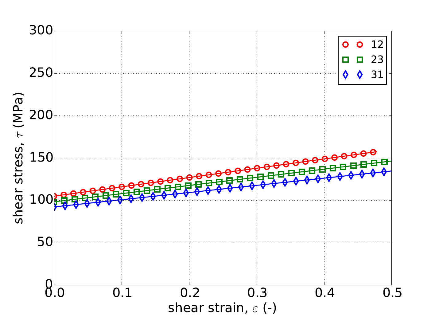
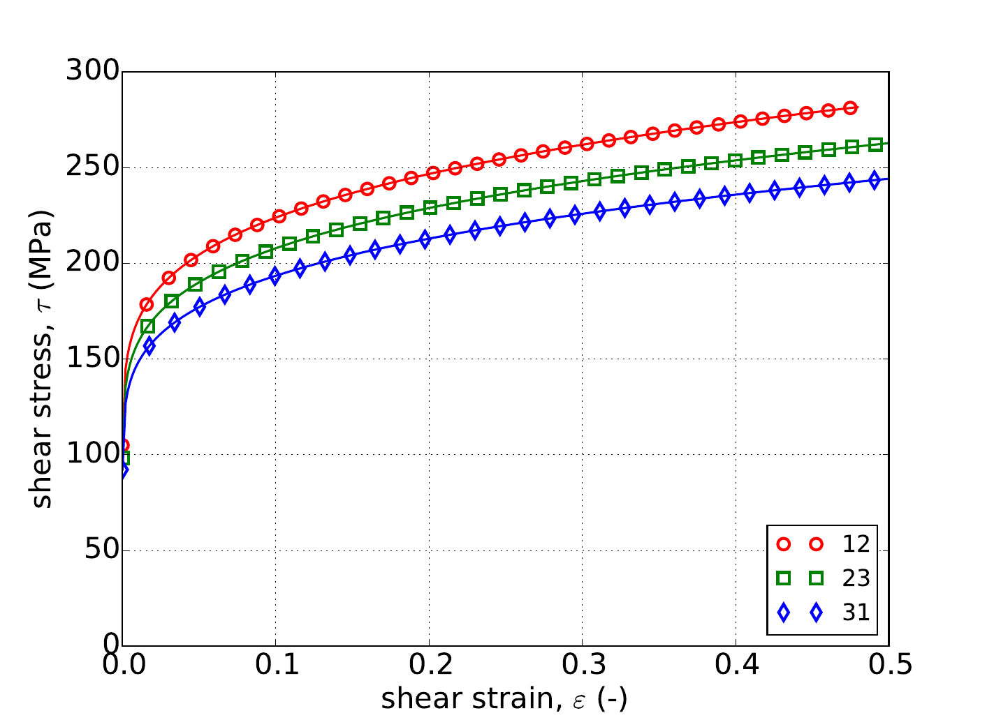
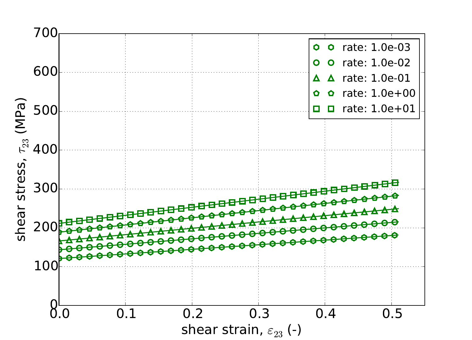
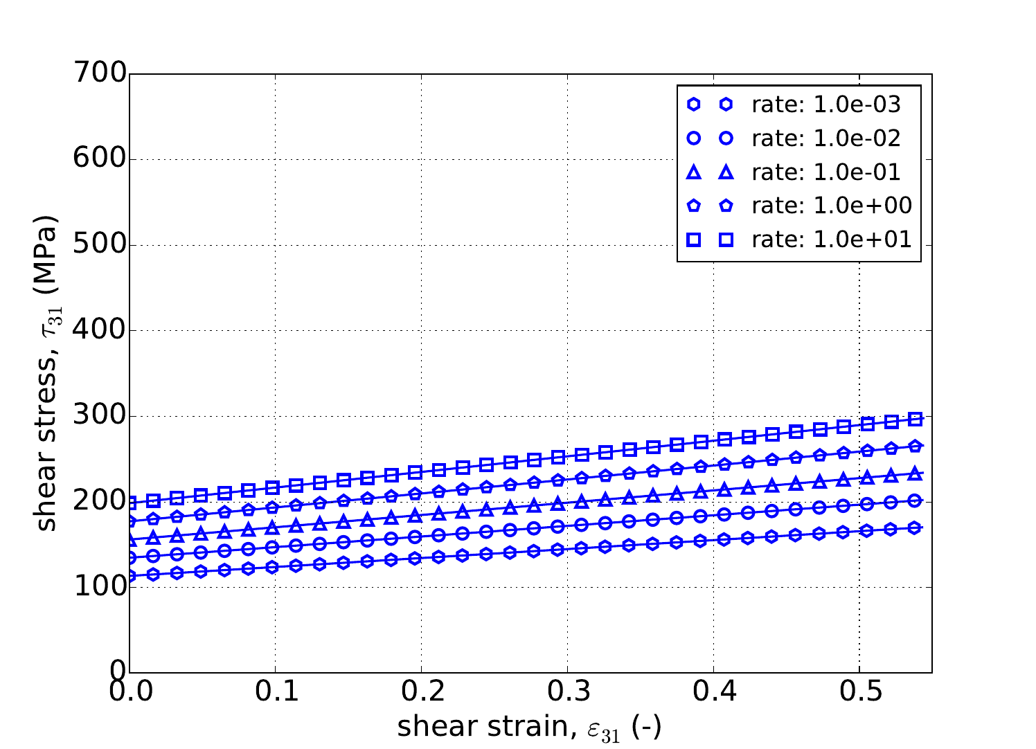
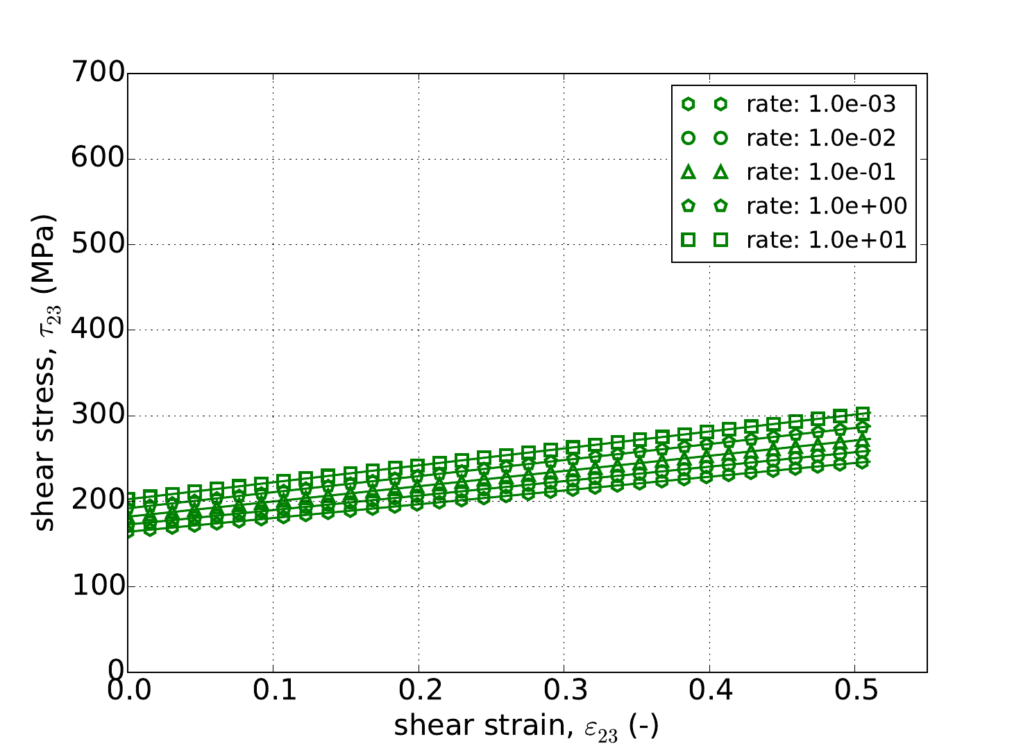
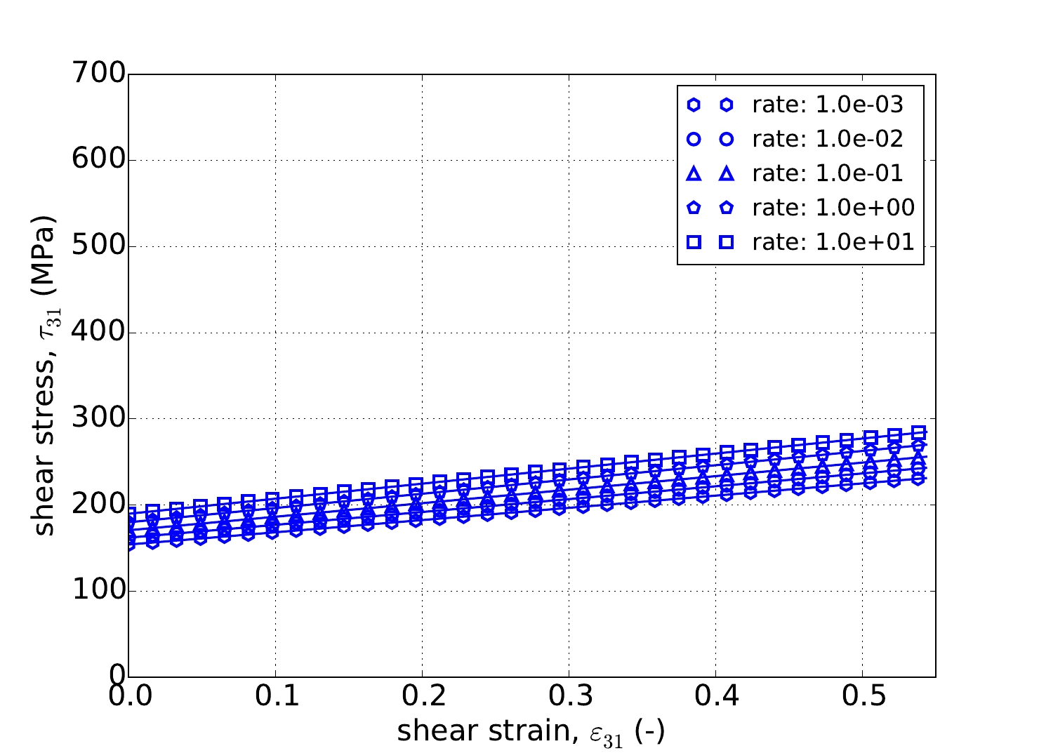
For the pure shear case, the problem discussed in Appendix A is considered. The results still depend on the Hill \(R\) coefficients and forty-five different loadings are presented in Fig. 4.69 and Fig. 4.70. In this instance, three different shearing planes are used in lieu of the principal directions. Nonetheless, for these results the key result remains the same – analytical matches numerical further verifying rate dependent capabilities.

Linear Hardening -- 11

Linear Hardening -- 22

Linear Hardening -- 33

Power-Law Hardening -- 11

Power-Law Hardening -- 22

Power-Law Hardening -- 33

Fig. 4.69 Stress-strain response of the Hill plasticity model with rate dependent, Johnson-Cook type hardening in pure shear with (a-c) linear and (d-f) power-law rate independent hardening. Solid lines are analytical results while open symbols are numerical.

Voce Hardening -- 11

Voce Hardening -- 22

Voce Hardening -- 33

Fig. 4.70 Stress-strain response of the Hill plasticity model with rate dependent, Johnson-Cook type hardening in pure shear with (a-c) Voce rate independent hardening. Solid lines are analytical results while open symbols are numerical.

4.15.3.3.5. Power-Law Breakdown

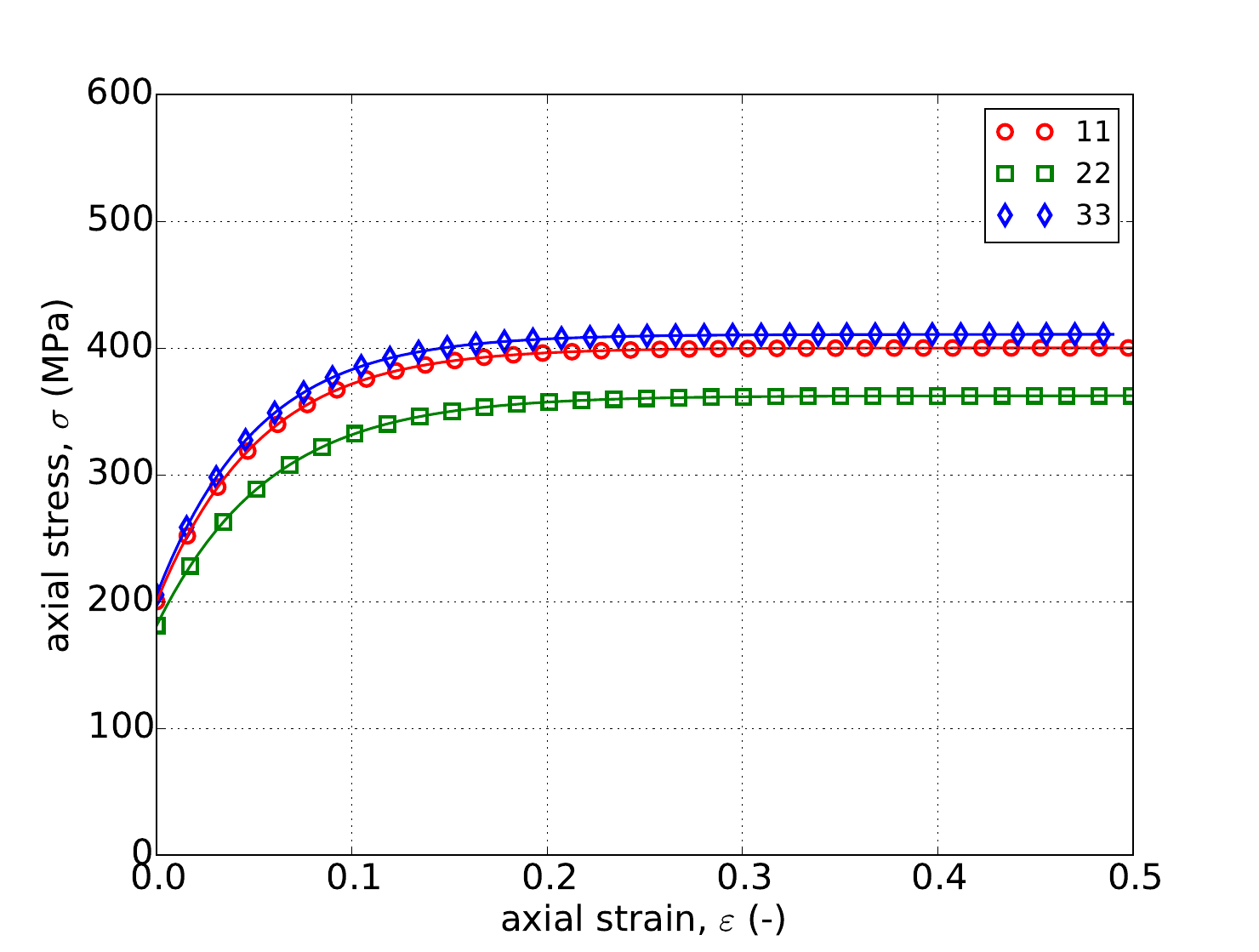
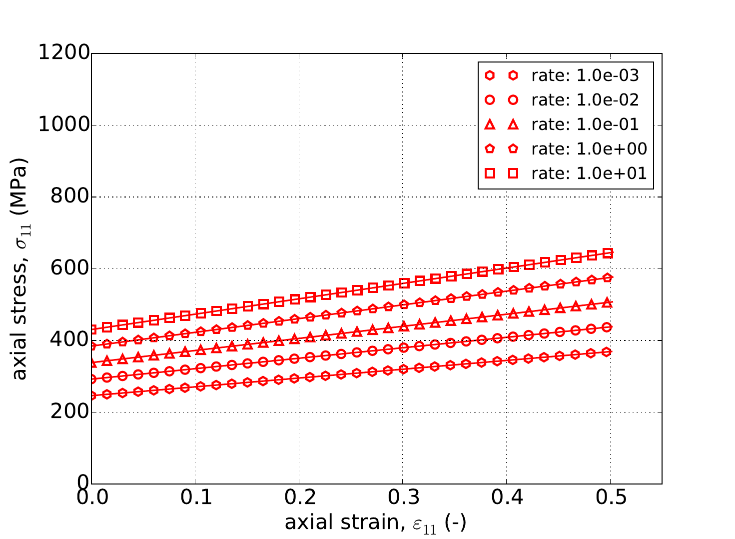
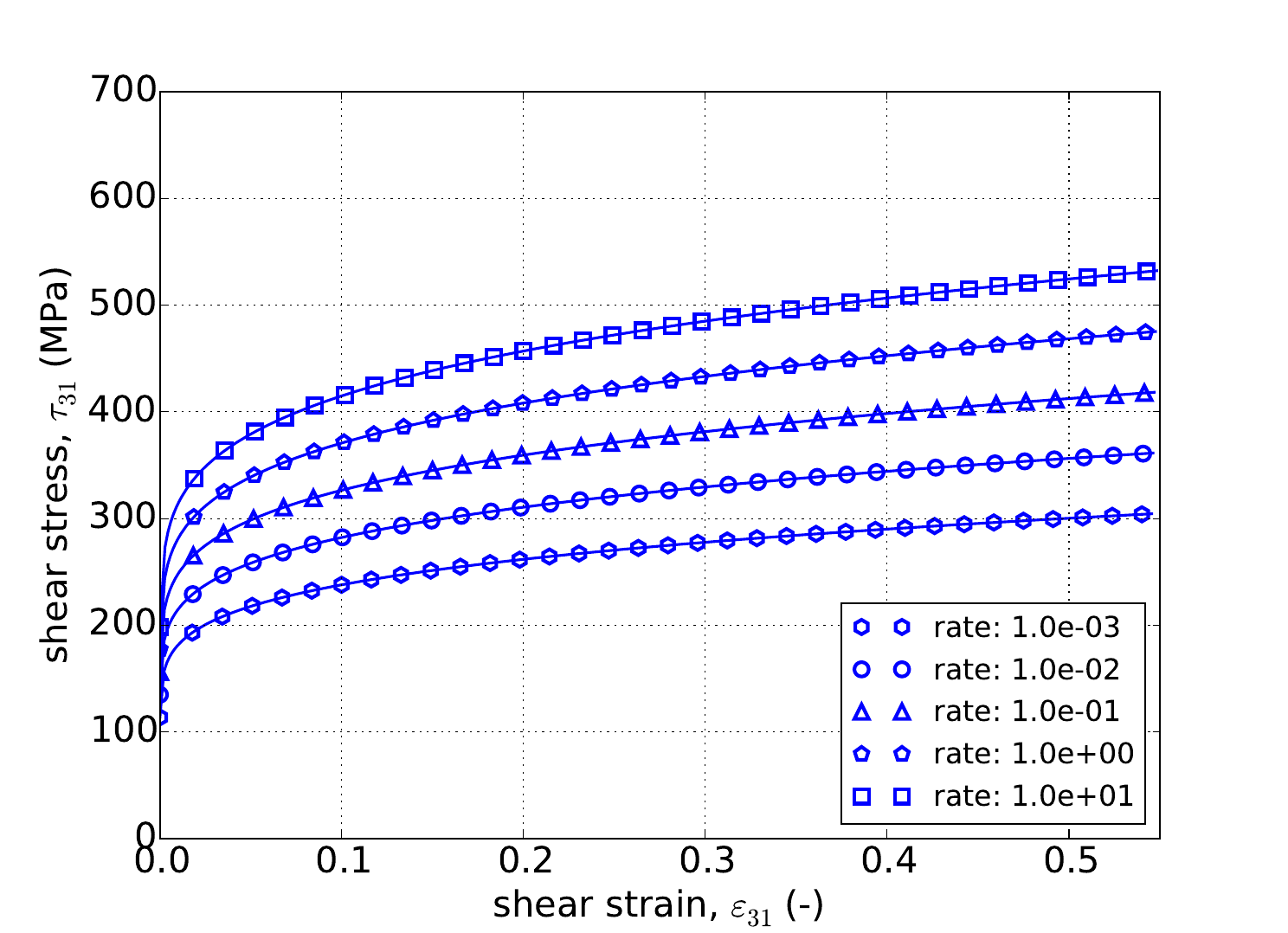
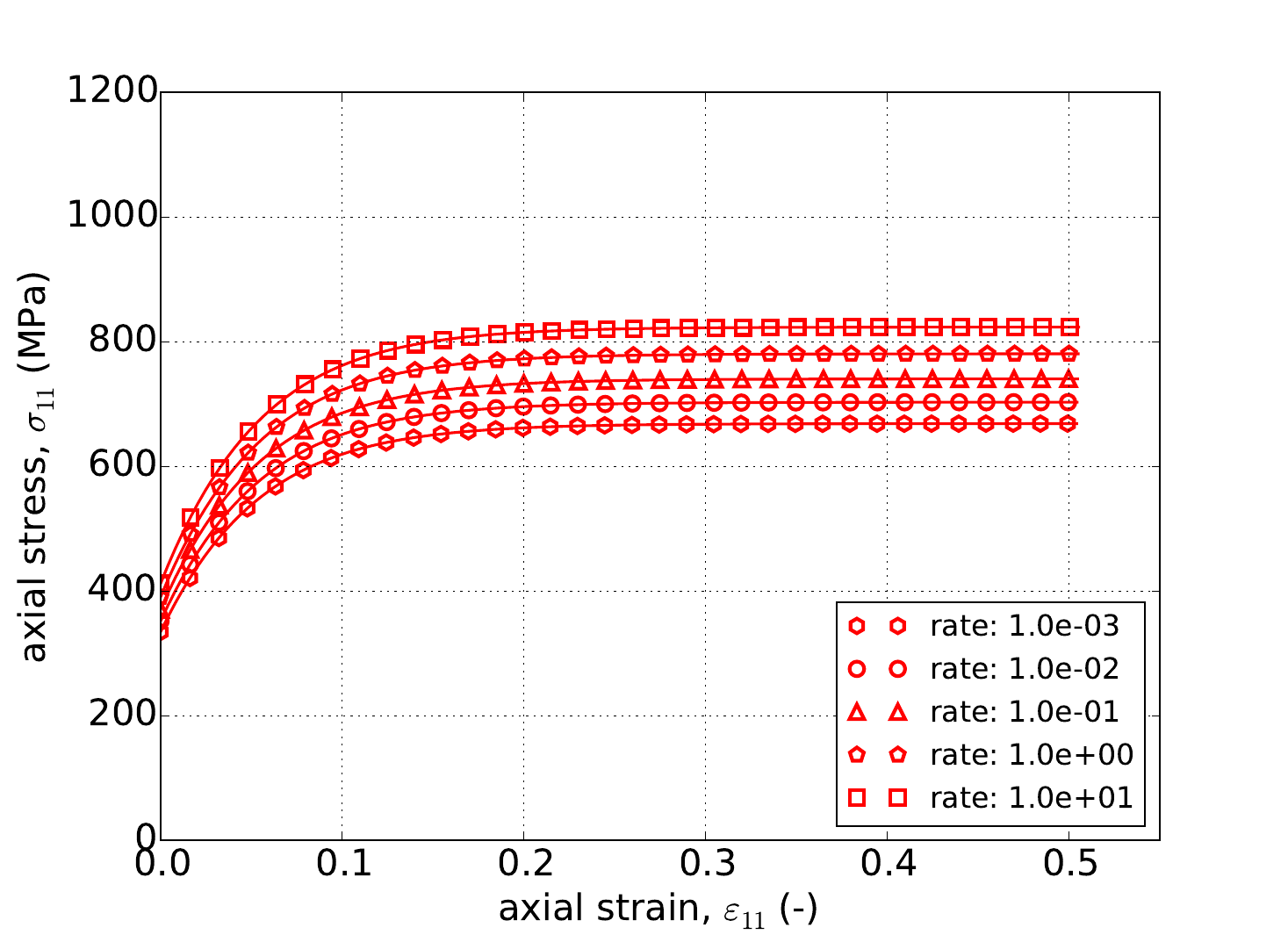
For the power-law breakdown model, the same forty-five cases discussed in the previous section (three directions, five rates, three hardening models) are again solved via the approach of Appendix A in Fig. 4.71 and Fig. 4.72. Although the impact of rate on the responses differs due to the assumed representation of the rate-dependent hardening, excellent agreement is still noted between analytical and numerical results.

Linear Hardening -- 11

Linear Hardening -- 22

Linear Hardening -- 33

Power-Law Hardening -- 11

Power-Law Hardening -- 22

Power-Law Hardening -- 33

Fig. 4.71 Uniaxial stress-strain response of the Hill plasticity model with rate dependent, power-law breakdown type hardening in with (a-c) linear and (d-f) power-law rate independent hardening. Solid lines are analytical results while open symbols are numerical.

Voce Hardening -- 11

Voce Hardening -- 22

Voce Hardening -- 33

Fig. 4.72 Uniaxial stress-strain response of the Hill plasticity model with rate dependent, power-law breakdown type hardening in with (a-c) Voce rate independent hardening. Solid lines are analytical results while open symbols are numerical.

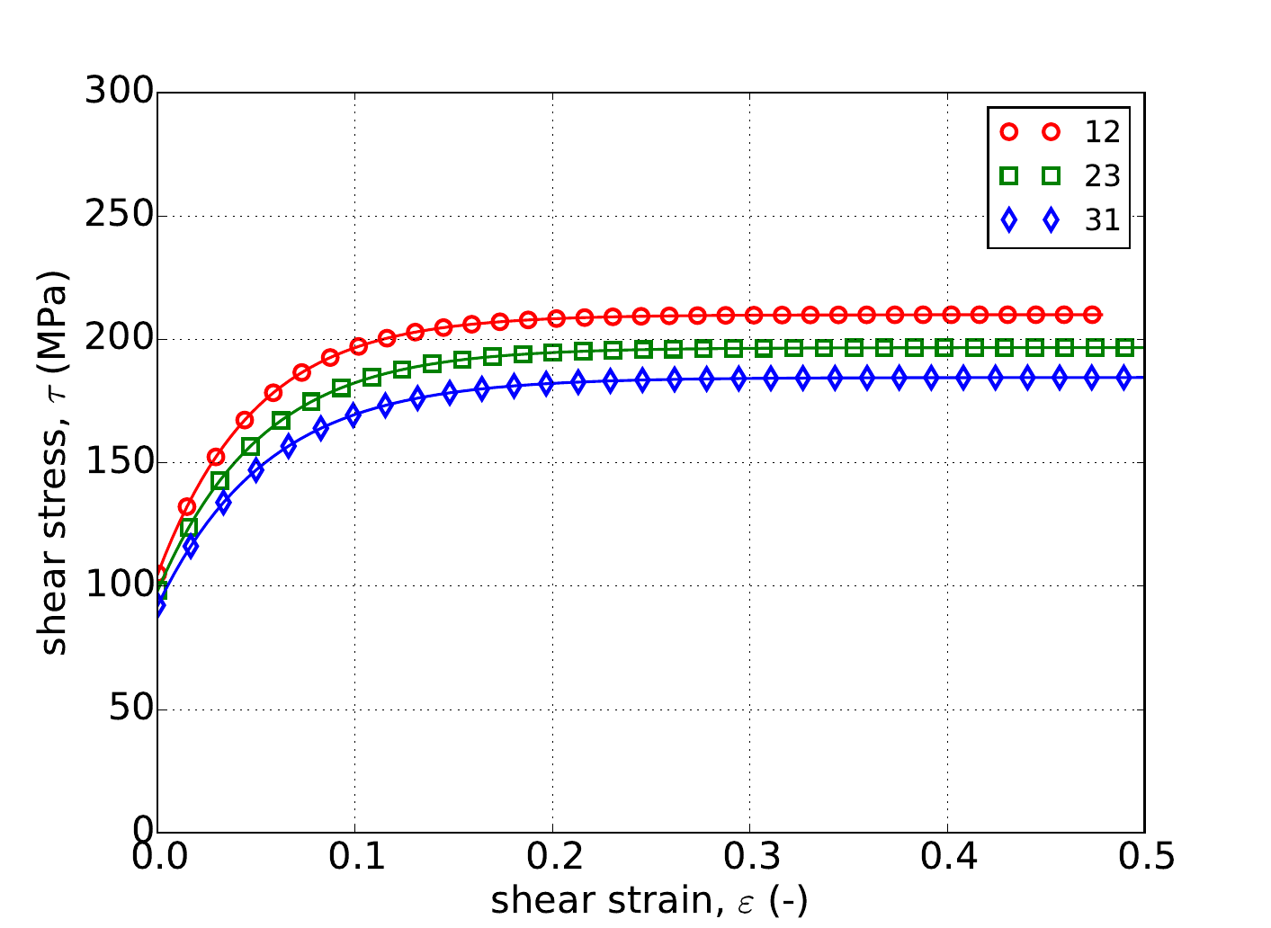
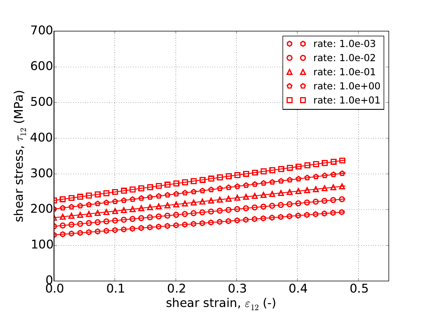
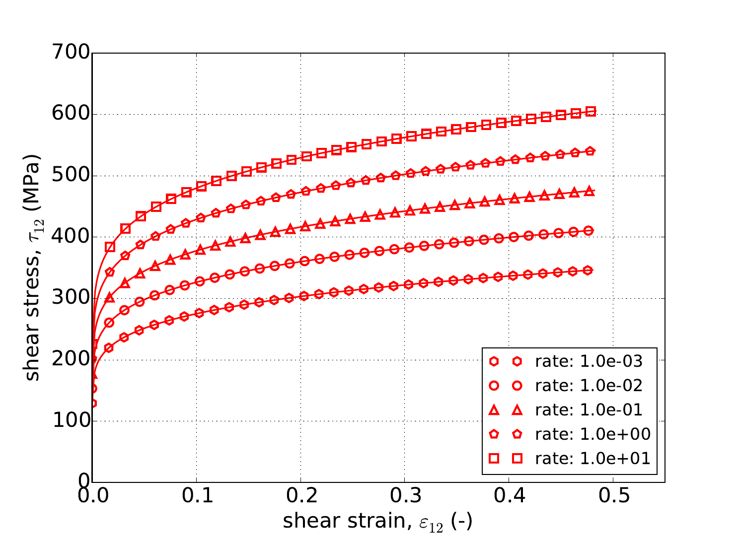
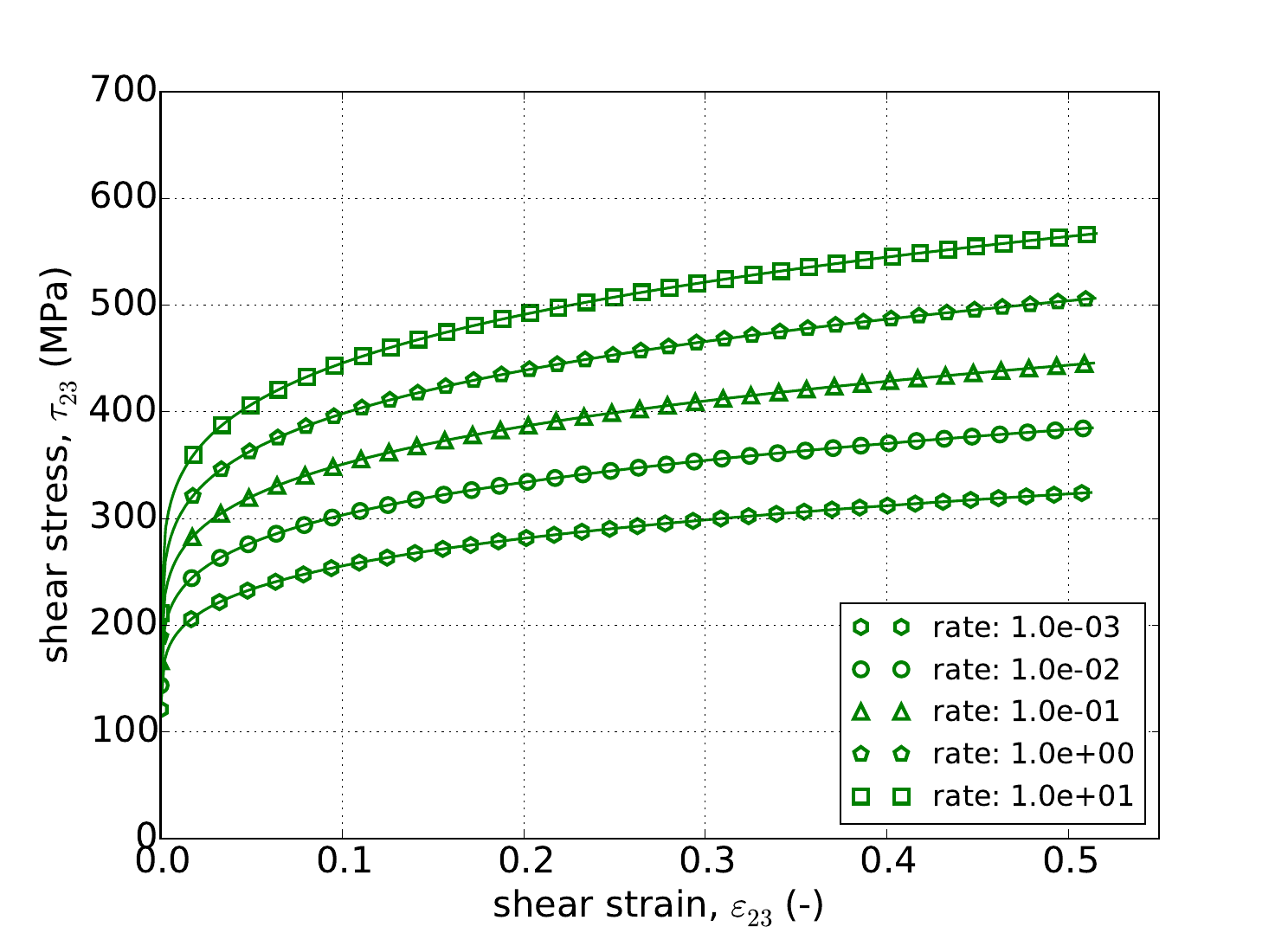
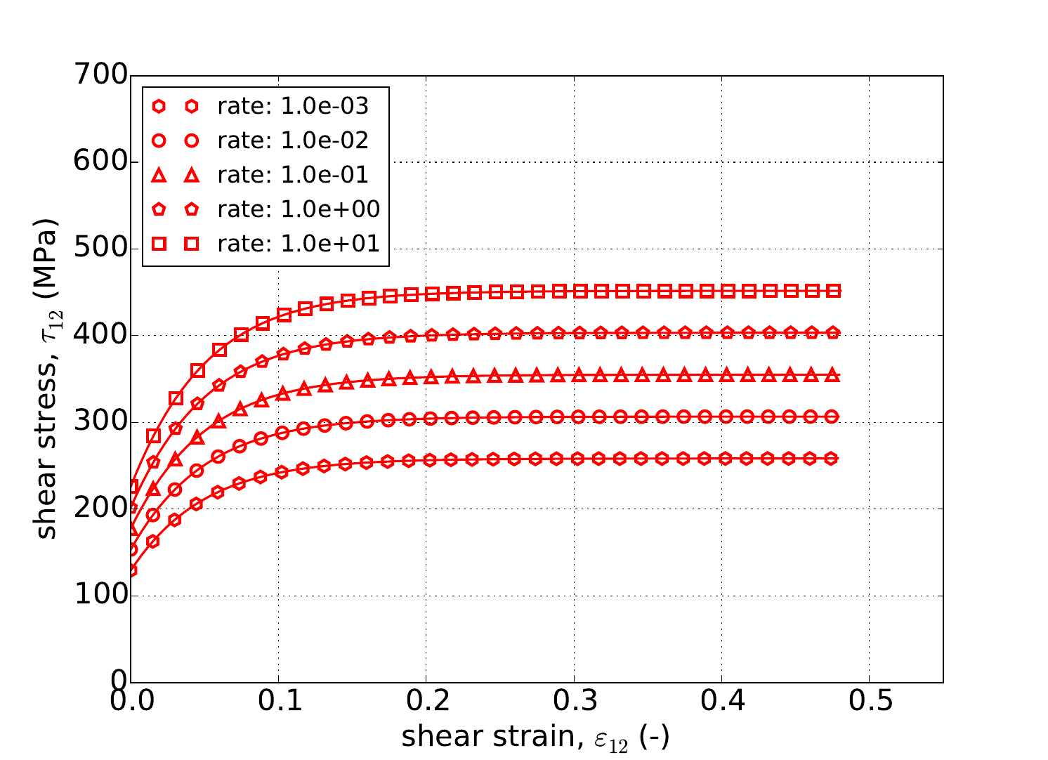
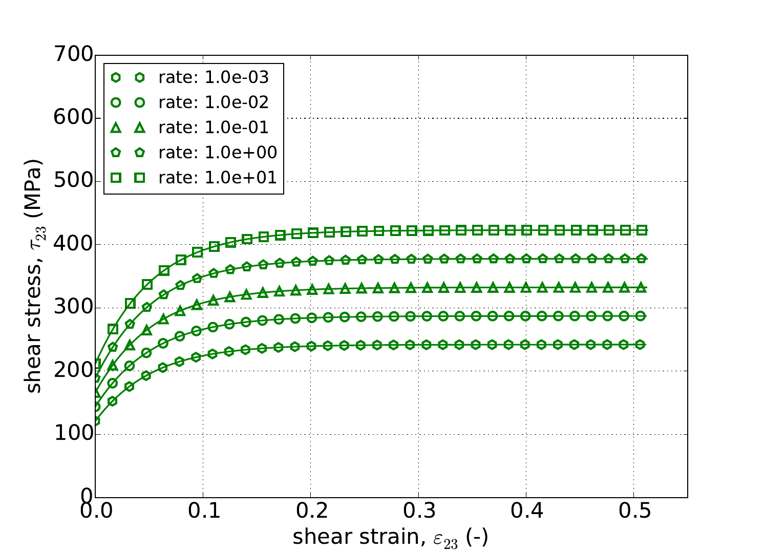
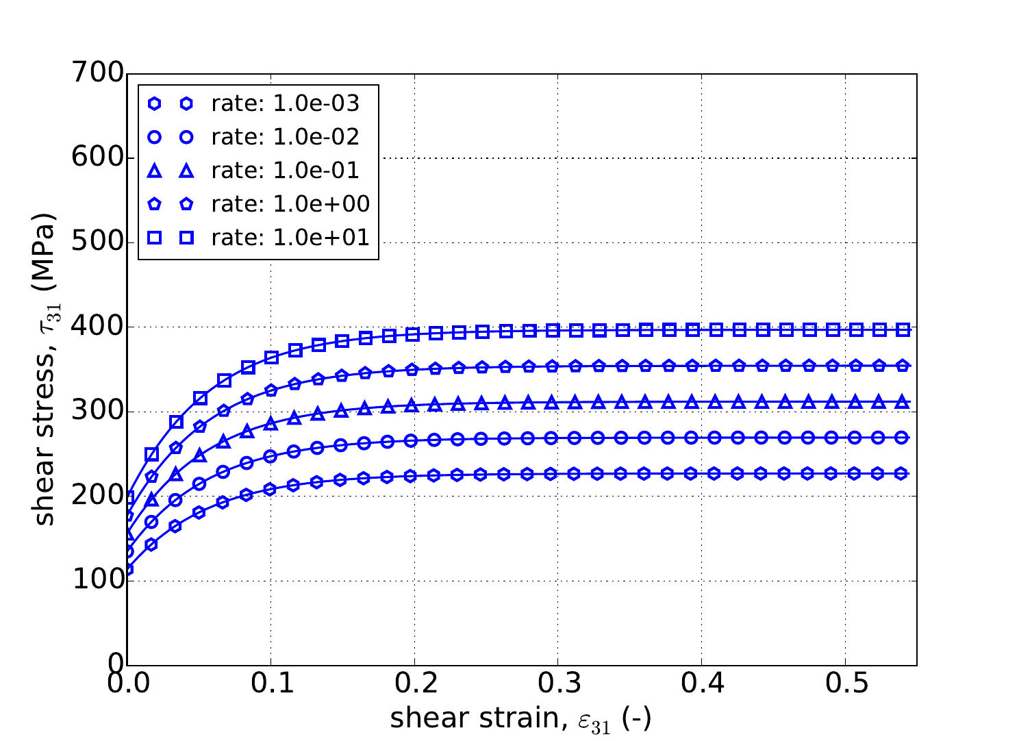
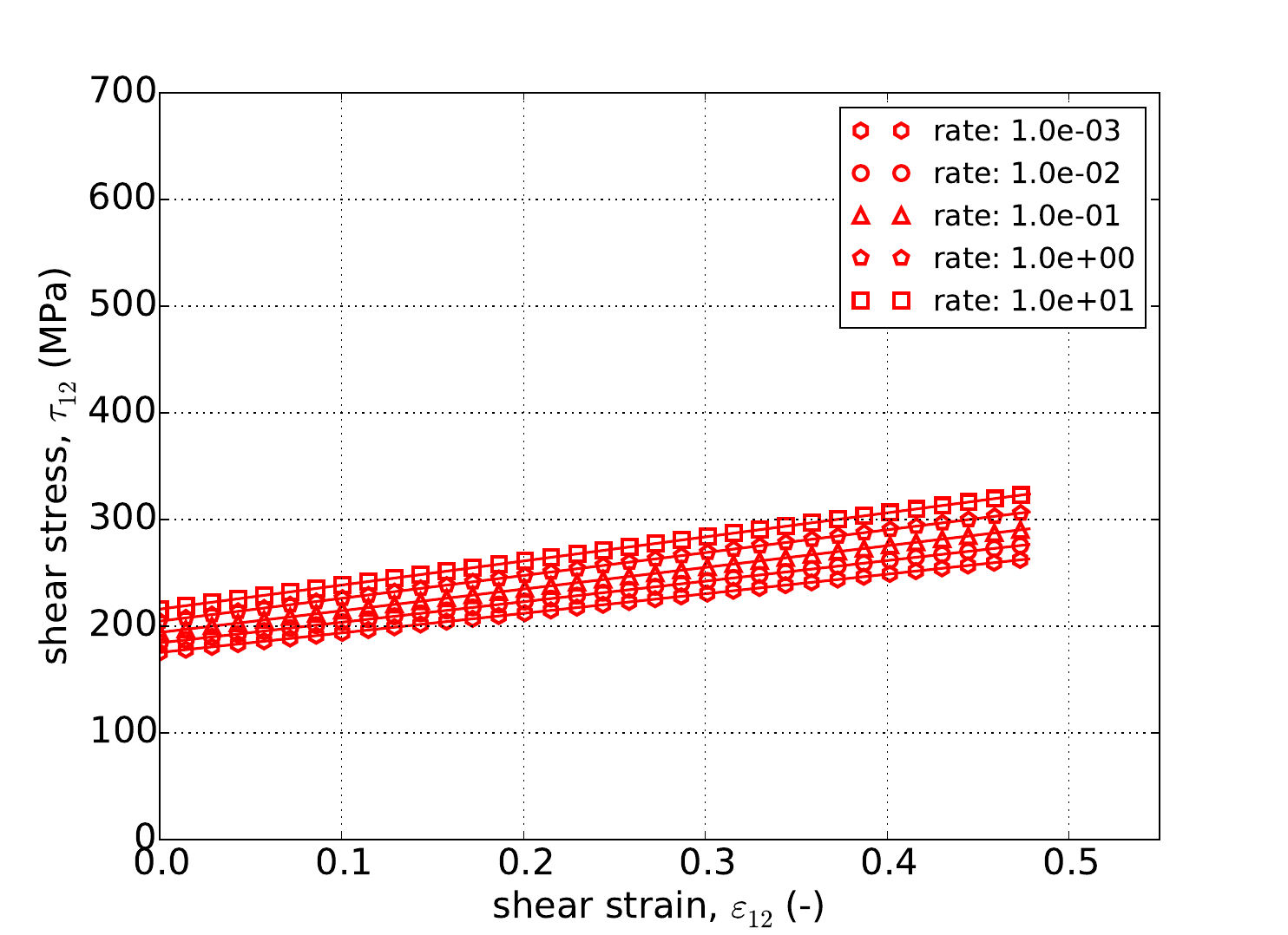
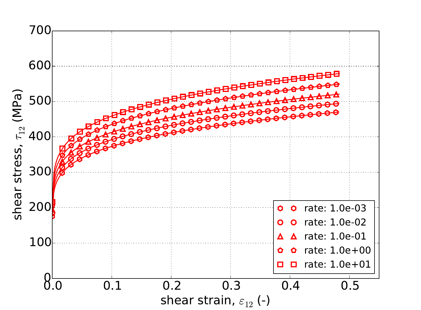
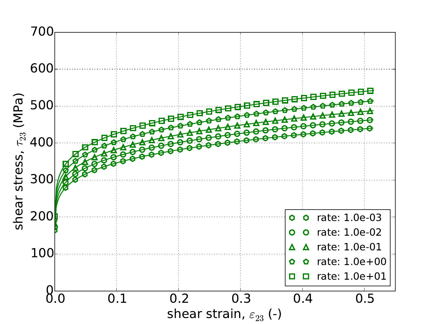
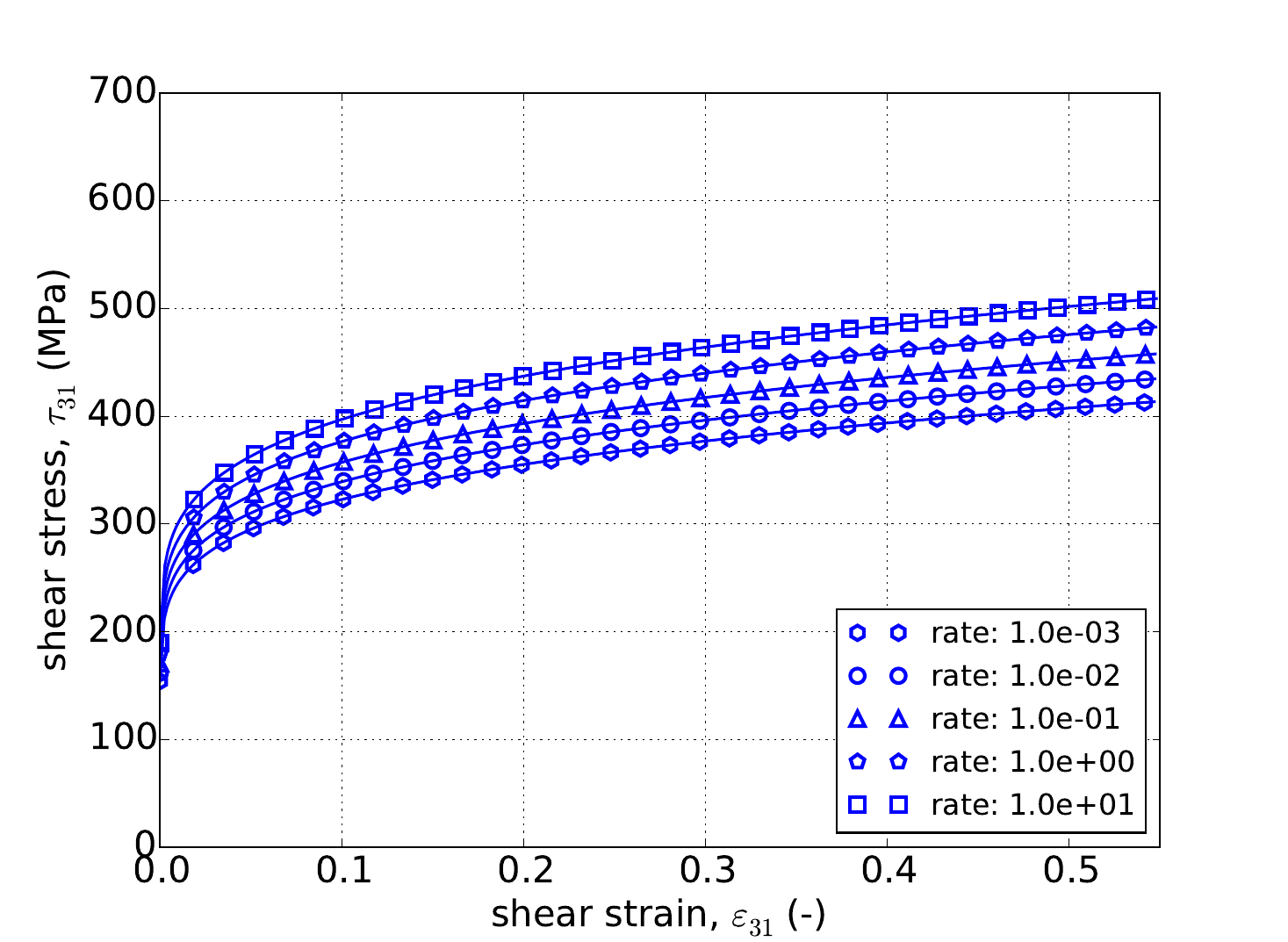
To expand on the uniaxial stress results, the response through pure shear is also probed via the method of Appendix A. Again forty-five different cases are investigated and their results are presented in Fig. 4.73 and Fig. 4.74. Once again, the results aligning thereby verifying the capability of the model and producing additional credibility.

Linear Hardening -- 11

Linear Hardening -- 22

Linear Hardening -- 33

Power-Law Hardening -- 11

Power-Law Hardening -- 22

Power-Law Hardening -- 33

Fig. 4.73 Stress-strain response of the Hill plasticity model with rate dependent, power-law breakdown type hardening in pure shear with (a-c) linear and (d-f) power-law rate independent hardening. Solid lines are analytical results while open symbols are numerical.

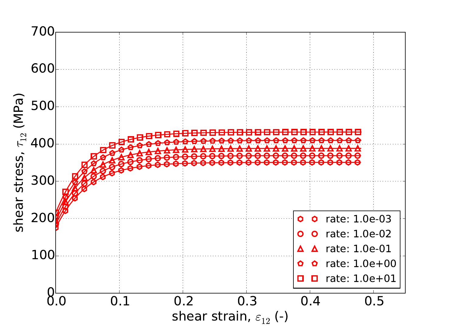Voce Hardening -- 11

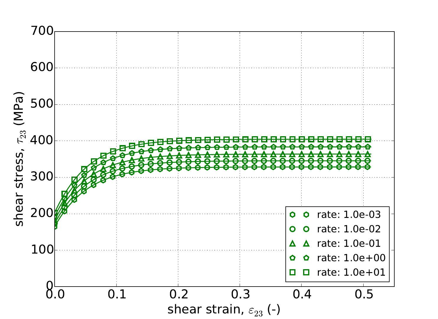Voce Hardening -- 22

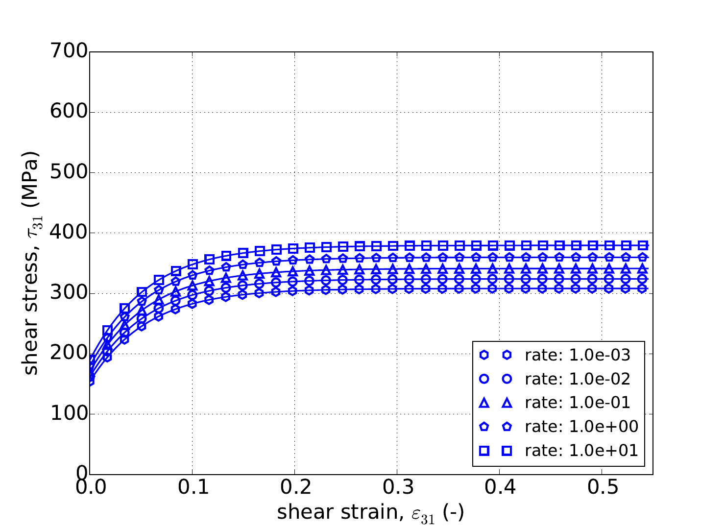Voce Hardening -- 33

Fig. 4.74 Stress-strain response of the Hill plasticity model with rate dependent, power-law breakdown type hardening in pure shear with (a-c) Voce rate independent hardening. Solid lines are analytical results while open symbols are numerical.

4.15.4. User Guide

BEGIN PARAMETERS FOR MODEL HILL_PLASTICITY
  #
  # Elastic constants
  #
  YOUNGS MODULUS = <real>
  POISSONS RATIO = <real>
  SHEAR MODULUS  = <real>
  BULK MODULUS   = <real>
  LAMBDA         = <real>
  TWO MU         = <real>
  #
  # Material coordinates system definition
  #
  COORDINATE SYSTEM             = <string> coordinate_system_name
  DIRECTION FOR ROTATION        = <real> 1|2|3
  ALPHA                         = <real> (degrees)
  SECOND DIRECTION FOR ROTATION = <real> 1|2|3
  SECOND ALPHA                  = <real> (degrees)
  #
  # Yield surface parameters
  #
  YIELD STRESS = <real>
  R11 = <real> (1.0)
  R22 = <real> (1.0)
  R33 = <real> (1.0)
  R12 = <real> (1.0)
  R23 = <real> (1.0)
  R31 = <real> (1.0)

#
  #
  # Hardening model
  #
  HARDENING MODEL = LINEAR | POWER_LAW | VOCE | USER_DEFINED |
  FLOW_STRESS | DECOUPLED_FLOW_STRESS | JOHNSON_COOK |
  POWER_LAW_BREAKDOWN
  #
  # Linear hardening
  #
  HARDENING MODULUS = <real>
  #
  # Power-law hardening
  #
  HARDENING CONSTANT = <real>
  HARDENING EXPONENT = <real> (0.5)
  LUDERS STRAIN      = <real> (0.0)
  #
  # Voce hardening
  #
  HARDENING MODULUS       = <real>
  EXPONENTIAL COEFFICIENT = <real>
  #
  # Johnson-Cook hardening
  #
  HARDENING FUNCTION = <string>hardening_function_name
  RATE CONSTANT      = <real>
  REFERENCE RATE     = <real>
  #
  # Power law breakdown hardening
  #
  HARDENING FUNCTION = <string>hardening_function_name
  RATE COEFFICIENT   = <real>
  RATE EXPONENT      = <real>
  # User defined hardening
  #
  HARDENING FUNCTION = <string>hardening_function_name
  #

#
  #
  # Following Commands Pertain to Flow_Stress Hardening Model
  #
  #    -  Isotropic Hardening model
  #
  ISOTROPIC HARDENING MODEL = LINEAR | POWER_LAW | VOCE |
                              USER_DEFINED
  #
  # Specifications for Linear, Power-law, and Voce same as above
  #
  # User defined hardening
  #
  ISOTROPIC HARDENING FUNCTION = <string>iso_hardening_fun_name
  #
  #     - Rate dependence
  #
  RATE MULTIPLIER = JOHNSON_COOK | POWER_LAW_BREAKDOWN |
     USER_DEFINED | RATE_INDEPENDENT (RATE_INDEPENDENT)
  #
  # Specifications for Johnson-Cook, Power-law-breakdown
  #     same as before EXCEPT no need to specify a
  #     hardening function
  #
  # User defined rate multiplier
  #
  RATE MULTIPLIER FUNCTION = <string> rate_mult_function_name
  #
  #     - Temperature dependence
  #
  TEMPERATURE MULTIPLIER = JOHNSON_COOK | USER_DEFINED |
     TEMPERATURE_INDEPENDENT (TEMPERATURE_INDEPENDENT)
  #
  #  Johnson-Cook temperature dependence
  #
  MELTING TEMPERATURE   = <real>
  REFERENCE TEMPERATURE = <real>
  TEMPERATURE EXPONENT  = <real>
  #
  #  User-defined temperature dependence
  TEMPERATURE MULTIPLIER FUNCTION = <string>temp_mult_function_name
  #
  # Following Commands Pertain to Decoupled_Flow_Stress Hardening Model
  #
  #    -  Isotropic Hardening model
  #
  ISOTROPIC HARDENING MODEL = LINEAR | POWER_LAW | VOCE | USER_DEFINED
  #
  # Specifications for Linear, Power-law, and Voce same as above
  #
  # User defined hardening
  #
  ISOTROPIC HARDENING FUNCTION = <string>isotropic_hardening_function_name
  #
  #     - Rate dependence
  #
  YIELD RATE MULTIPLIER = JOHNSON_COOK | POWER_LAW_BREAKDOWN |
              USER_DEFINED | RATE_INDEPENDENT (RATE_INDEPENDENT)
  #
  # Specifications for Johnson-Cook, Power-law-breakdown same as before
  #     EXCEPT no need to specify a hardening function
  #     AND should be preceded by YIELD
  #
  #     As an example for Johnson-Cook yield rate dependence,
  #
  YIELD RATE CONSTANT  = <real>
  YIELD REFERENCE RATE = <real>
  #
  # User defined rate multiplier
  #
  YIELD RATE MULTIPLIER FUNCTION = <string>yield_rate_mult_function_name
  #
  HARDENING_RATE MULTIPLIER = JOHNSON_COOK | POWER_LAW_BREAKDOWN |
              USER_DEFINED | RATE_INDEPENDENT (RATE_INDEPENDENT)
  #
  #     Syntax same as for yield parameters but with a HARDENING prefix
  #
  #     - Temperature dependence
  #
  YIELD TEMPERATURE MULTIPLIER = JOHNSON_COOK | USER_DEFINED |
            TEMPERATURE_INDEPENDENT (TEMPERATURE_INDEPENDENT)
  #
  #  Johnson-Cook temperature dependence
  #
  YIELD MELTING TEMPERATURE   = <real>
  YIELD REFERENCE TEMPERATURE = <real>
  YIELD TEMPERATURE EXPONENT  = <real>
  #
  #  User-defined temperature dependence
  YIELD TEMPERATURE MULTIPLIER FUNCTION = <string>yield_temp_mult_fun_name
  #
  HARDENING TEMPERATURE MULTIPLIER = JOHNSON_COOK | USER_DEFINED |
            TEMPERATURE_INDEPENDENT (TEMPERATURE_INDEPENDENT)
  #
  #   Syntax for hardening constants same as for yield but
  #            with HARDENING prefix

#
  #
  # Optional Failure Definitions
  #    Following only need to be defined if intend to use failure model
  #
  FAILURE MODEL = TEARING_PARAMETER | JOHNSON_COOK_FAILURE | WILKINS
                  | MODULAR_FAILURE | MODULAR_BCJ_FAILURE

  CRITICAL FAILURE PARAMETER = <real>
  #
  # TEARING_PARAMETER Failure model definitions
  #
  TEARING PARAMETER EXPONENT = <real>
  #
  # JOHNSON_COOK_FAILURE Failure model definitions
  #
  JOHNSON COOK D1       = <real>
  JOHNSON COOK D2       = <real>
  JOHNSON COOK D3       = <real>
  JOHNSON COOK D4       = <real>
  JOHNSON COOK D5       = <real>
  #
  #Following Johnson-Cook parameters can only be defined once.  As such, only
  #  needed if not previously defined via Johnson-Cook multipliers
  #  w/ flow-stress hardening.  Does need to be defined
  #  w/ Decoupled Flow Stress
  #
  REFERENCE RATE        = <real>
  REFERENCE TEMPERATURE = <real>
  MELTING TEMPERATURE   = <real>
  #
  # WILKINS Failure model definitions
  #
  WILKINS ALPHA    = <real>
  WILKINS BETA     = <real>
  WILKINS PRESSURE = <real>
  #
  #  MODULAR_FAILURE Failure model definitions
  #
  PRESSURE MULTIPLIER         = PRESSURE_INDEPENDENT | WILKINS
                                | USER_DEFINED (PRESSURE_INDEPENDENT)
  LODE ANGLE MULTIPLIER       = LODE_ANGLE_INDEPENDENT |
                                WILKINS (LODE_ANGLE_INDEPENDENT)
  TRIAXIALITY MULTIPLIER      = TRIAXIALITY_INDEPENDENT | JOHNSON_COOK
                                | USER_DEFINED (TRIAXIALITY_INDEPENDENT)
  RATE FAIL MULTIPLIER        = RATE_INDEPENDENT | JOHNSON_COOK
                                | USER_DEFINED (RATE_INDEPENDENT)
  TEMPERATURE FAIL MULTIPLIER = TEMPERATURE_INDEPENDENT | JOHNSON_COOK
                                | USER_DEFINED (TEMPERATURE_INDEPENDENT)
  #
  # Individual multiplier definitions
  #
  PRESSURE MULTIPLIER = WILKINS
  WILKINS ALPHA       = <real>
  WILKINS PRESSURE    = <real>
  #
  PRESSURE MULTIPLIER = USER_DEFINED
  PRESSURE MULTIPLIER FUNCTION = <string> pressure_multiplier_fun_name
  #
  LODE ANGLE MULTIPLIER = WILKINS
  WILKINS BETA          = <real>
  #
  TRIAXIALITY MULTIPLIER = JOHNSON_COOK
  JOHNSON COOK D1        = <real>
  JOHNSON COOK D2        = <real>
  JOHNSON COOK D3        = <real>
  #
  TRIAXIALITY MULTIPLIER = USER_DEFINED
  TRIAXIALITY MULTIPLIER FUNCTION = <string> triaxiality_multiplier_fun_name
  #
  RATE FAIL MULTIPLIER = JOHNSON_COOK
  JOHNSON COOK D4      = <real>
  # REFERENCE RATE should only be added if not previously defined
  REFERENCE RATE       = <real>
  #
  RATE FAIL MULTIPLIER = USER_DEFINED
  RATE FAIL MULTIPLIER FUNCTION = <string> rate_fail_multiplier_fun_name
  #
  TEMPERATURE FAIL MULTIPLIER = JOHNSON_COOK
  JOHNSON COOK D5             = <real>
  # JC Temperatures should only be defined if not previously given
  REFERENCE TEMPERATURE       = <real>
  MELTING TEMPERATURE         = <real>
  #
  TEMPERATURE FAIL MULTIPLIER          = USER_DEFINED
  TEMPERATURE FAIL MULTIPLIER FUNCTION = <string> temp_multiplier_fun_name
  #
  # MODULAR_BCJ_FAILURE Failure model definitions
  #
  INITIAL DAMAGE    = <real>
  INITIAL VOID SIZE = <real>
  DAMAGE BETA       = <real> (0.5)
  GROWTH MODEL      = COCKS_ASHBY | NO_GROWTH (NO_GROWTH)
  NUCLEATION MODEL  = HORSTEMEYER_GOKHALE | CHU_NEEDLEMAN_STRAIN
                      | NO_NUCLEATION (NO_NUCLEATION)
  #
  GROWTH RATE FAIL MULTIPLIER        = JOHNSON_COOK | USER_DEFINED
                                       | RATE_INDEPENDENT
                                       (RATE_INDEPENDENT)
  GROWTH TEMPERATURE FAIL MULTIPLIER = JOHNSON_COOK | USER_DEFINED
                                       | TEMPERATURE_INDEPENDENT
                                       (TEMPERATURE_INDEPENDENT)
  #
  NUCLEATION RATE FAIL MULTIPLIER        = JOHNSON_COOK | USER_DEFINED
                                           | RATE_INDEPENDENT
                                           (RATE_INDEPENDENT)
  NUCLEATION TEMPERATURE FAIL MULTIPLIER = JOHNSON_COOK | USER_DEFINED
                                           | TEMPERATURE_INDEPENDENT
                                           (TEMPERATURE_INDEPENDENT)
  #
  # Definitions for individual growth and nucleation models
  #
  GROWTH MODEL = COCKS_ASHBY
  DAMAGE EXPONENT = <real> (0.5)
  #
  NUCLEATION MODEL      = HORSTEMEYER_GOKHALE
  NUCLEATION PARAMETER1 = <real> (0.0)
  NUCLEATION PARAMETER2 = <real> (0.0)
  NUCLEATION PARAMETER3 = <real> (0.0)
  #
  NUCLEATION MODEL          = CHU_NEEDLEMAN_STRAIN
  NUCLEATION AMPLITUDE      = <real>
  MEAN NUCLEATION STRAIN    = <real>
  NUCLEATION STRAIN STD DEV = <real>
  #
  # Definitions for rate and temperature fail multiplier
  #   Note: only showing definitions for growth.
  #    Nucleation terms are the same just with NUCLEATION instead
  #    of GROWTH
  #
  GROWTH RATE FAIL MULTIPLIER = JOHNSON_COOK
  GROWTH JOHNSON COOK D4      = <real>
  GROWTH REFERENCE RATE       = <real>
  #
  GROWTH RATE FAIL MULTIPLIER          = USER_DEFINED
  GROWTH RATE FAIL MULTIPLIER FUNCTION = <string> growth_rate_fail_mult_func
  #
  GROWTH TEMPERATURE FAIL MULTIPLIER = JOHNSON_COOK
  GROWTH JOHNSON COOK D5             = <real>
  GROWTH REFERENCE TEMPERATURE       = <real>
  GROWTH MELTING TEMPERATURE         = <real>
  #
  GROWTH TEMPERATURE FAIL MULTIPLIER          = USER_DEFINED
  GROWTH TEMPERATURE FAIL MULTIPLIER FUNCTION = <string> temp_fail_mult_func
  #

#
  #
  # Optional Adiabatic Heating/Thermal Softening  Definitions
  #    Following only need to be defined if intend to use failure model
  #
  THERMAL SOFTENING MODEL = ADIABATIC | COUPLED
  #
  SPECIFIC HEAT = <real> # not needed for COUPLED
  BETA_TQ       = <real>

END [PARAMETERS FOR MODEL HILL_PLASTICITY]

In the command blocks that define the Hill plasticity model:

• The reference nominal yield stress, \(\bar{\sigma}\), is defined with the YIELD STRESS command line.

• The ratio of the normal yield stress in the \(\bar{\bf e}_{1}\bar{\bf e}_{1}\) material direction is defined with the R11 command line. The default is 1.0.

• The ratio of the normal yield stress in the \(\bar{\bf e}_{2}\bar{\bf e}_{2}\) material direction is defined with the R22 command line. The default is 1.0.

• The ratio of the normal yield stress in the \(\bar{\bf e}_{3}\bar{\bf e}_{3}\) material direction is defined with the R33 command line. The default is 1.0.

• The ratio of the shear yield stress in the \(\bar{\bf e}_{1}\bar{\bf e}_{2}\) material direction is defined with the R12 command line. The default is 1.0.

• The ratio of the shear yield stress in the \(\bar{\bf e}_{2}\bar{\bf e}_{3}\) material direction is defined with the R23 command line. The default is 1.0.

• The ratio of the shear yield stress in the \(\bar{\bf e}_{3}\bar{\bf e}_{1}\) material direction is defined with the R31 command line. The default is 1.0.

• The type of hardening law is defined with the HARDENING MODEL command line, other hardening commands then define the specific shape of that hardening curve.

• The hardening modulus for a linear hardening model is defined with the HARDENING MODULUS command line.

• The hardening constant for a power law hardening model is defined with the HARDENING CONSTANT command line.

• The hardening exponent for a power law hardening model is defined with the HARDENING EXPONENT command line.

• The Luders strain for a power law hardening model is defined with the LUDERS STRAIN command line.

• The hardening function for a user defined hardening model is defined with the HARDENING FUNCTION command line.

• The shape of the spline for the spline based hardening is defined by the CUBIC SPLINE TYPE, CARDINAL PARAMETER, KNOT EQPS, and KNOT STRESS command lines.

Output variables available for this model are listed in Table 4.21.

Table 4.21 State Variables for HILL PLASTICITY Model

Name	Description
EQPS	equivalent plastic strain, \(\bar{\varepsilon}^{p}\)
EQDOT	equivalent plastic strain rate, \(\dot{\bar{\varepsilon}}^{p}\)
SEFF	effective stress, \(\phi\)
TENSILE_EQPS	tensile equivalent plastic strain, \(\bar{\varepsilon}^{p}_{t}\)
DAMAGE	damage, \(\phi\)
VOID_COUNT	void count, \(\eta\)
VOID_SIZE	void size, \(\upsilon\)
DAMAGE_DOT	damage rate, \(\dot{\phi}\)
VOID_COUNT_DOT	void count rate, \(\dot{\eta}\)
PLASTIC_WORK_HEAT_RATE	plastic work heat rate, \(\dot{Q}^p\)

---

[1]

W. M. Scherzinger. A return mapping algorithm for isotropic and anisotropic plasticity models using a line search method. Computer Methods in Applied Mechanics and Engineering, 317:526–553, 2017.

[2] (1,2)

R. Hill. The Mathematical Theory of Plasticity. Oxford University Press, 1950.

[3] (1,2)

B.T. Lester and W.M. Scherzinger. Failure formulations in modular plasticity models. Memo to distribution SAND2019-9678R, Sandia National Laboratories, Albuquerque, NM and Livermore, CA, 2019.

[4] (1,2)

B.T. Lester and W.M. Scherzinger. Modular growth and nucleation formulations in modular plasticity models. Memo to distribution SAND2020-7404R, Sandia National Laboratories, Albuquerque, NM and Livermore, CA, 2020.

[5] (1,2)

B.T. Lester and W.M. Scherzinger. Adiabatic heating in modular plasticity models. Memo to distribution SAND2019-15003R, Sandia National Laboratories, Albuquerque, NM and Livermore, CA, 2019.

[6]

J. Lemaitre and J.-L. Chaboche. Mechanics of Solid Materials. Cambridge University Press, 1990.

[7]

J. Lubliner. Plasticity Theory. Dover, 2008.

[8] (1,2,3,4,5)

G.R. Johnson and W.H. Cook. A constitutive model and data for metals subjected to large strains, high strain rates and high temperatures. In Proc. 7th. Int. Symp. on Ballistics, 541–547. The Hague, The Netherlands, 1983.

[9] (1,2,3,4,5)

G.R. Johnson and W.H. Cook. Fracture characteristics of three metals subjected to various strains, strain rates, temperatures and pressures. Engineering Fracture Mechanics, 21(1):31–48, 1985.

[10]

H. J. Frost and M. F. Ashby. Deformation Mechanism Maps: the Plasticity and Creep of Metals and Ceramics. Pergamon Press, 1982.

[11]

A.A. Brown and D.J. Bammann. Validation of a model for static and dynamic recrystallization in metals. International Journal of Plasticity, 32–33:17–35, 2012.

[12]

F. Barlat, H. Aretz, J. W. Yoon, J. C. Brem, and R. E. Dick. Linear transformation-based anisotropic yield functions. International Journal of Plasticity, 21:1009–1039, 2005.