4.36. Phase Field F^eF^p Model

Phase Field F^eF^p is an implementation of a cohesive variational phase-field fracture model developed for the purpose of modeling brittle and ductile fracture. The model is based upon the F^eF^p model, a hyperelastic analogue of the J₂ plasticity model, and features a von-Mises yield surface and isotropic hardening. Phase Field F^eF^p is meant to be used in conjunction with a phase-field solver. The use of Sierra/SM’s reaction-diffusion solver is strongly recommended. The model leverages several of LAMÉ’s modular hardening capabilities, specifically those for which hardening potentials have been defined: linear, power-law, and Voce hardening. Rate-dependent and temperature-dependent plasticity are not yet implemented for this model.

4.36.1. Theory

4.36.1.1. Overview

An overview of the Phase Field F^eF^p model theory is presented in this section. For more comprehensive analytical derivations for this model, we refer the interested reader to the following references: [[1], [2], [3]].

The phase-field fracture model derives from the Griffith brittle fracture model, characterized by a fracture energy release rate \(G_c\). In that framework, the solution to the fracture mechanics problem can be cast as the minimum of a free energy functional, with displacements \(u\) and state variables \(z\):

(4.231)\[\psi^* = \min_{u,z,\Gamma} \left( \int_{\Omega} \psi^m(u,z) \,\mathrm{d}\Omega\, + \int_{\Gamma} G_c \,\mathrm{d}\Gamma\, \right),\]

where \(\psi^m\) is the mechanical energy potential (traditionally elastic strain energy). The phase-field model approximates the discrete crack on surface \(\Gamma\) as a smeared continuum damage field in volume \(\Omega\) using the phase field \(\phi\), as illustrated in Fig. 4.154 adapted from [[4]].

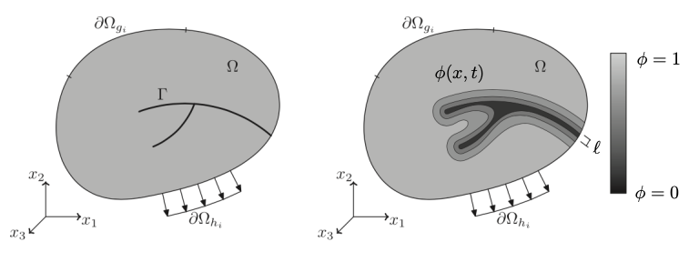
Fig. 4.154 Approximation of sharp crack by smeared phase field.

The material coherence convention is used here, where \(\phi = 1\) refers to intact material, and \(\phi = 0\) refers to completely damaged material. The mechanical energy potential is degraded through a degradation function \(g(\phi)\), defined such that \(g(1) = 1\) and \(g(0) = 0\). Note that some references use variable \(c\) for this interpretation of the phase field; other references interpret the phase field as damage, increasing from zero to one as the material degrades, \(d = 1-\phi\).

We impose the following constraints on the phase field, representing that it remains within the physical range and that damage is irreversible:

\[\begin{split}\begin{cases} 0 \leq \phi \leq 1 \\ \dot{\phi} \leq 0 \end{cases}.\end{split}\]

The problem solution is therefore recast in terms of this approximation:

(4.232)\[\psi = \int_{\Omega} \psi^m(u,z,\phi) + G_c \psi^f(\phi, \nabla{\phi}, \ell) \,\mathrm{d}\Omega\,,\]

(4.233)\[\psi^* = \min_{u,z,\phi} \psi,\]

with \(\psi^f\) representing a fracture energy or damage potential that includes a regularizing length scale \(\ell\). The approximation (4.232) is \(\Gamma\)-convergent to the original functional (4.231) in the limit \(\ell \rightarrow 0\). The mechanical energy is degraded through the application of individual degradation functions for each the elastic and plastic components:

\[\begin{split}\begin{cases} \psi^m(u,z,\phi) = \psi^e(u,z,\phi) + \psi^p(z,\phi) \\ \psi^e(u,z,\phi) = {g^e}(\phi) \widetilde{\psi}^e(u,z) \\ \psi^p(z,\phi) = {g^p}(\phi) \widetilde{\psi}^p(z) \end{cases} .\end{split}\]

In order to provide an asymmetric response between tension and compression, an additional modification is made to the elastic energy potential \(\widetilde{\psi}^e\), decomposing it into a positive portion \(\widetilde{\psi}^e_+\) that can damage and a negative portion \(\widetilde{\psi}^e_-\) that cannot: \(\widetilde{\psi}^e = \widetilde{\psi}^e_+ + \widetilde{\psi}^e_-\). The degradation functions are applied only to the positive portion:

\[\psi^e(u,z,\phi) = {g^e}(\phi) \widetilde{\psi}^e_+(u,z) + \widetilde{\psi}^e_-(u,z) .\]

Details of the elastic potential, plastic potentials, damage potentials, degradation functions, and tension-compression splits are provided in subsequent sections: Section 4.36.1.2, Section 4.36.2, Section 4.36.2.2, Section 4.36.2.3, Section 4.36.2.4.

To provide a direct energetic basis for the phase-field model, the Phase Field F^eF^p model is implemented with a hyperelastic formulation. Therefore, the kinematics of plastic deformation are written in terms of the deformation gradient \(F\), which is multiplicatively decomposed into elastic (\({F^e}\)) and plastic (\({F^p}\)) components:

\[F = {F^e} {F^p}.\]

The deformation gradient \(F_{n+1}\) at each timestep is taken as an input for the model, while the plastic deformation gradient \({F^p}\) is initialized as identity and maintained as a state variable. These key variables take the place of the previously-defined displacement \(u\) and state variable \(z\), respectively. The elastic deformation gradient is therefore defined as \({F^e} = F {F^p}^{-1}\), and the plastic flow rule \(\dot{F^p} {F^p}^{-1} = {{}\dot{\bar{\varepsilon}}^p} N^p\), with equivalent plastic strain rate \({{}\dot{\bar{\varepsilon}}^p}\) and flow direction tensor \(N^p\).

The equations of motion for this material model derive from the Euler-Lagrange equations that correspond to the stationary point of the energy Lagrangian \(\mathcal{L}\) (given the irreversibility of plasticity and damage, the equations of motion actually derive from finding the stationary point of an incremental Lagrangian, \((\delta \mathcal{L})_{n+1} (u, z, \phi) = \mathcal{L}_{n+1} - \mathcal{L}_{n}\), with \(\mathcal{L}_{n}\) fixed and \(F_{n+1}(u_{n+1})\) known.). The Lagrangian is formed using the free energy functional \(\psi\) and power from applied loads \(L\) (\(b_0\) refers to a prescribed body force per unit volume, \({\chi} = \frac{\partial x}{\partial X}\) is the deformation map, \(\bar{t}_0\) is a Neumann traction boundary condition, and \(\bar{\xi}_0\) is Neumann phase boundary condition [not commonly used]):

\[L = \int_{\Omega} b_0 \cdot \dot{{\chi}} \,\mathrm{d}\Omega\, + \int_{\partial_{t} \Omega} \bar{t}_0 \cdot \dot{{\chi}} \,\mathrm{d}\partial \Omega\, + \int_{\partial_{\xi} \Omega} \bar{\xi}_0 \dot{\phi} \,\mathrm{d}\partial \Omega\, ,\]

\[\mathcal{L} = \psi - L ,\]

(4.234)\[\begin{split}\begin{cases} \nabla\cdot \frac{\partial \mathcal{L} }{\partial \nabla{u} } - \frac{\partial \mathcal{L}}{\partial u} & = 0 \\ \nabla\cdot \frac{\partial \mathcal{L}}{\partial \nabla{z} } - \frac{\partial \mathcal{L}}{\partial z} & = 0 \\ \nabla\cdot \frac{\partial \mathcal{L} }{\partial \nabla{\phi} } - \frac{\partial \mathcal{L}}{\partial \phi} & = 0 \end{cases} .\end{split}\]

The Euler-Lagrange equations (4.234) simplify to the usual balance of linear momentum for solid mechanics with Piola-Kirchoff stress \(P\) and boundary normal \(n_0\)

(4.235)\[\begin{split}\begin{cases} \nabla\cdot P + b_0 = 0 & \mbox{in } \Omega \\ P \cdot n_0 = \bar{t}_0 & \mbox{on } \partial_{t} \Omega \end{cases},\end{split}\]

a plastic yield surface that corresponds to a damaged version of the familiar \(J_2\) von-Mises yield surface with quasistatic flow stress \(Y^{\mathrm{eq}}\) when corresponding constraints on the flow tensor \(N^p\) are applied (\(N^p : N^p = \frac32\), \(\mathrm{tr}(N^p) =0\))

(4.236)\[\begin{split}\begin{cases} \left( \bar{\sigma} = \sqrt{\frac32} \left\|\mathrm{dev}{\sigma}\right\| = \sqrt{\frac32} {g^e}(\phi) \left\|\mathrm{dev}\frac{\partial \widetilde{\psi}^e_+}{\partial {\varepsilon^{e}}}\right\| \right) = \left( Y^{\mathrm{eq}} = {g^p}(\phi) \frac{\partial\widetilde{\psi}^p}{\partial\bar{\varepsilon}^p} \right) \\ N^p = \sqrt{\frac32} \frac{ \mathrm{dev}{\sigma} }{\left\|\mathrm{dev}{\sigma}\right\|} \end{cases},\end{split}\]

and reveal the phase-field update equation

(4.237)\[\begin{split}\begin{cases} \frac{\partial \psi^f}{\partial \nabla{\phi}} G_c - \frac{\partial{g^e}}{\partial\phi} \widetilde{\psi}^e_+ - \frac{\partial {g^p}}{\partial \phi} \widetilde{\psi}^p - \frac{\partial \psi^f}{\partial \phi} G_c = 0 & \mbox{in } \Omega \\ \frac{\partial \psi^f}{\partial \nabla{\phi}} \cdot n_0 = \bar{\xi}_0 & \mbox{on } \partial_{\xi} \Omega \end{cases}.\end{split}\]

For the classical phase-field fracture model (AT-2, e.g. [[5], [6], [7]]), this update equation is

(4.238)\[2 G_c \ell \Delta \phi - 2 \phi \left( \widetilde{\psi}^e_+ + \widetilde{\psi}^p \right) + \frac{G_c}{2\ell} (1-\phi) = 0,\]

and for the threshold model (AT-1, e.g. [[8]]), the update equation is

(4.239)\[\frac{3 G_c \ell}{4} \Delta \phi - 2 \phi \left( \widetilde{\psi}^e_+ + \widetilde{\psi}^p \right) + \frac{3 G_c}{8 \ell} = 0.\]

The phase field update is generally a non-linear reaction-diffusion partial differential equation of the form \(R(\phi) - D \Delta \phi = S\), whereas (4.238) and (4.239) are linear: \(R \phi - D \Delta \phi = S\). Casting the equation into this form enables solution through familiar algorithms in Sierra. This is detailed in Section 4.36.4.2.

Details of the implemented elastic potentials, plastic potentials, damage potentials, and degradation functions follow:

4.36.1.2. Elastic Potential

Isotropic Hencky elasticity using logarithmic strain is selected for the elastic constitutive model. The logarithmic strain tensor is defined from the elastic deformation gradient:

\[{\varepsilon^{e}} = \frac{1}{2}\log({F^e}^T {F^e}).\]

The isotropic Hencky elastic potential is defined in terms of the logarithmic strain, as:

\[\widetilde{\psi}^e = \mu \mathrm{dev}({\varepsilon^{e}}):\mathrm{dev}({\varepsilon^{e}}) + \frac{\kappa}{2} \left( \mathrm{tr}( {\varepsilon^{e}}) \right)^2,\]

and the work-conjugate Mandel stress is defined as (this expression may be later modified by a tension-compression split)

\[\sigma^{M} = \frac{\partial \psi^e}{\partial {\varepsilon^{e}}} = {g^e}(\phi) \left( 2 \mu \mathrm{dev}({\varepsilon^{e}}) + \kappa \mathrm{tr}( {\varepsilon^{e}}) \right).\]

Cauchy stress can then be defined as:

\[\sigma = \frac{1}{J} {F^e}^{-T} \sigma^{M} {F^e}^T .\]

4.36.2. Plastic Hardening

4.36.2.1. Rate Sensitivity

The variational model proposed by Talamini et al. [[3]] provides for the possibility of rate-dependent plasticity through the inclusion of a dual kinetic potential \(\Pi^*({{}\dot{\bar{\varepsilon}}^p},\phi)\), with the requirement that its derivative approaches zero in the quasistatic limit (\({{}\dot{\bar{\varepsilon}}^p} \rightarrow 0^+\)). The dissipation potential identifies two components \(Y^{\mathrm{vis}}\) and \({{}\dot{\bar{\varepsilon}}^p}\) that define the total dissipation density \(\mathcal{D}\):

\[\mathcal{D} = Y^{\mathrm{vis}} {{}\dot{\bar{\varepsilon}}^p} ,\]

\[Y^{\mathrm{vis}} = \frac{\partial \Pi^*}{\partial {{}\dot{\bar{\varepsilon}}^p}} .\]

When rate-dependence is included in the formulation, the viscous over-stress \(Y^{\mathrm{vis}}\) would be added to the quasistatic flow stress \(Y^{\mathrm{eq}}\), replacing (4.236) with the following:

(4.240)\[\left( \bar{\sigma} = \sqrt{\frac32} \left\|\mathrm{dev}{\sigma}\right\| = \sqrt{\frac32} {g^e}(\phi) \left\|\mathrm{dev}\frac{\partial \widetilde{\psi}^e_+}{\partial {\varepsilon^{e}}}\right\| \right) = \left( Y^{\mathrm{eq}} = {g^p}(\phi) \frac{\partial \widetilde{\psi}^p}{\partial \bar{\varepsilon}^p} \right) + \left( Y^{\mathrm{vis}} = {g^p}(\phi) \frac{\partial \Pi^*}{\partial {{}\dot{\bar{\varepsilon}}^p}} \right) .\]

As an example, Hu et al. [[9]] proposes a power-law rate-sensitivity dissipation density of the form:

\[\Pi^* = \frac{m}{m+1} {Y_0} \dot{\epsilon}_0 \left( \frac{{{}\dot{\bar{\varepsilon}}^p}}{\dot{\epsilon}_0} \right) ^{(m+1)/m}\]

Rate-dependent plasticity has not yet been implemented into Phase Field F^eF^p to date.

4.36.2.2. Damage Potentials

The damage potential implemented for Phase Field F^eF^p is the so-called AT-1 potential that includes a linear term in phase:

(4.241)\[\psi^f = \frac{3}{8 \ell} \left( (1-\phi) + \ell^2 \nabla \phi \cdot \nabla \phi \right)\]

This damage potential was first proposed by Pham et al. [[8]] and is a critical component of the so-called threshold models, named because this potential gives rise to a critical energy threshold \(\psi_c\) which must be reached before damage begins evolving. The critical energy threshold can be revealed by substituting this damage potential into (4.237):

\[\frac{3 G_c \ell}{4} \Delta \phi - \frac{\partial {g^e}}{\partial \phi} \widetilde{\psi}^e_+ - \frac{\partial {g^p}}{\partial \phi} \widetilde{\psi}^p + \frac{3 G_c}{8 \ell} = 0 .\]

For a uniformly intact initial state, the phase field is defined as \(\phi=1\) and \(\Delta \phi = 0\). The condition required to evolve beyond this state corresponds to:

(4.242)\[\frac{\partial {g^e}}{\partial \phi} \widetilde{\psi}^e_+ + \frac{\partial {g^p}}{\partial \phi} \widetilde{\psi}^p = \frac{3 G_c}{8 \ell} .\]

When combined with the common quadratic degradation function (4.244), \({g^e}(\phi)={g^p}(\phi)={g^{\text{Q}}}(\phi)\), this reduces to

(4.243)\[\psi_c = \left( \widetilde{\psi}^e_+ + \widetilde{\psi}^p \right)_c = \frac{3 G_c}{16 \ell}\]

4.36.2.3. Degradation Functions

The most common degradation function found in the literature is the quadratic degradation function:

(4.244)\[{g^{\text{Q}}}(\phi) = \phi^2\]

When combined with the linear damage potential, this gives rise to the critical energy threshold described above (4.243). For a given load path, the critical energy threshold can be related to a critical failure strength. For example, for an elastic material (\(\widetilde{\psi}^p=0\)) under uniaxial tension, the driving energy is a function of the stress \(\widetilde{\psi}^e = \frac{\sigma^2}{2E}\), so the failure threshold can be found to be \(\sigma_c = \sqrt{\frac{3G_c E}{8\ell}}\). Therefore, the failure threshold (\(\psi_c\) or \(\sigma_c\)) depends on the phase field length scale \(\ell\). The length scale \(\ell\) serves as a numerical parameter, with the model convergent to Griffith fracture in the limit as \(\ell \rightarrow 0\), so the failure threshold approaches infinity. Alternatively, the length scale can be selected so that the critical stress matches the material failure stress [[8]].

In contrast, when modeling ductile failure, there exists a physical yield stress \({\text{R}}\). Now, the relationship between \(\sigma_c\) and the yield stress has consequence in terms of model physics. This can be recast in terms of length scales: the interaction between the magnitudes of the phase-field fracture length scale \(\ell\) and the plastic zone size \(r_p\). This means that the phase-field length scale is now effectively a material parameter, rather than a numerical one.

This was the motivation for the degradation function proposed by Talamini et al. [[3]]. This degradation function \(g^{\text{R}}(\phi)\) takes the form of a rational function and includes \(\psi_c\) as a new parameter:

(4.245)\[g^{\text{R}}(\phi) = \frac{\phi^2}{\left( 1 + \gamma (1-\phi) \right)^2} ,\]

(4.246)\[\gamma = \frac{3 G_c}{16 \ell \psi_c} - 1.\]

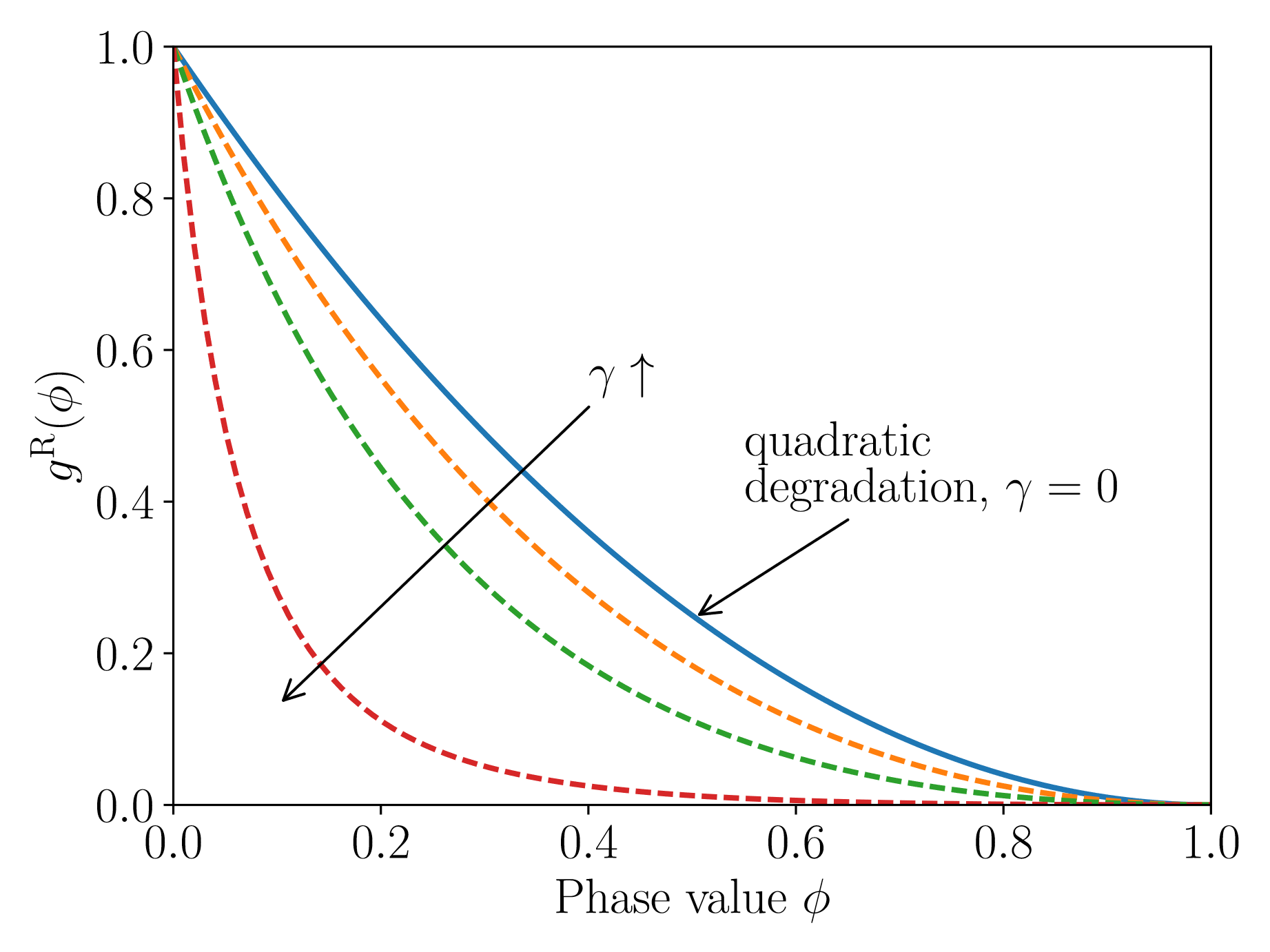
Fig. 4.155 Effect of parameter \(\gamma\) in the rational degradation function. Graphs are shown for \(\gamma = \lbrace 0, \tfrac{1}{3}, 1, 7 \rbrace\). Increasing \(\gamma\) makes the degradation function (and hence the stress) drop off more quickly with increasing phase value.

The effect of \(\gamma\) on the degradation behavior is shown in Fig. 4.155. In order to ensure convexity of the degradation function and solution uniqueness, a bound of \(\gamma \geq -\frac13\) is recommended; this corresponds to an upper bound for the threshold parameter: \(\psi_c \leq \frac{9 G_c}{32 \ell}\). The quadratic degradation function exists as a special case of this model, when \(\gamma = 0\), \(\psi_c = \frac{3 G_c}{16 \ell}\).

Repeating (4.242) and (4.243) using \(g^{\text{R}}(\phi)\) confirms that the new \(\psi_c\) parameter is returned as the effective critical energy threshold. This restores the interpretation of \(\ell\) as a numerical parameter. The effect of degradation function parameters \(\psi_c\) and \(\gamma\), is demonstrated on uniaxial constitutive response in Fig. 4.156.

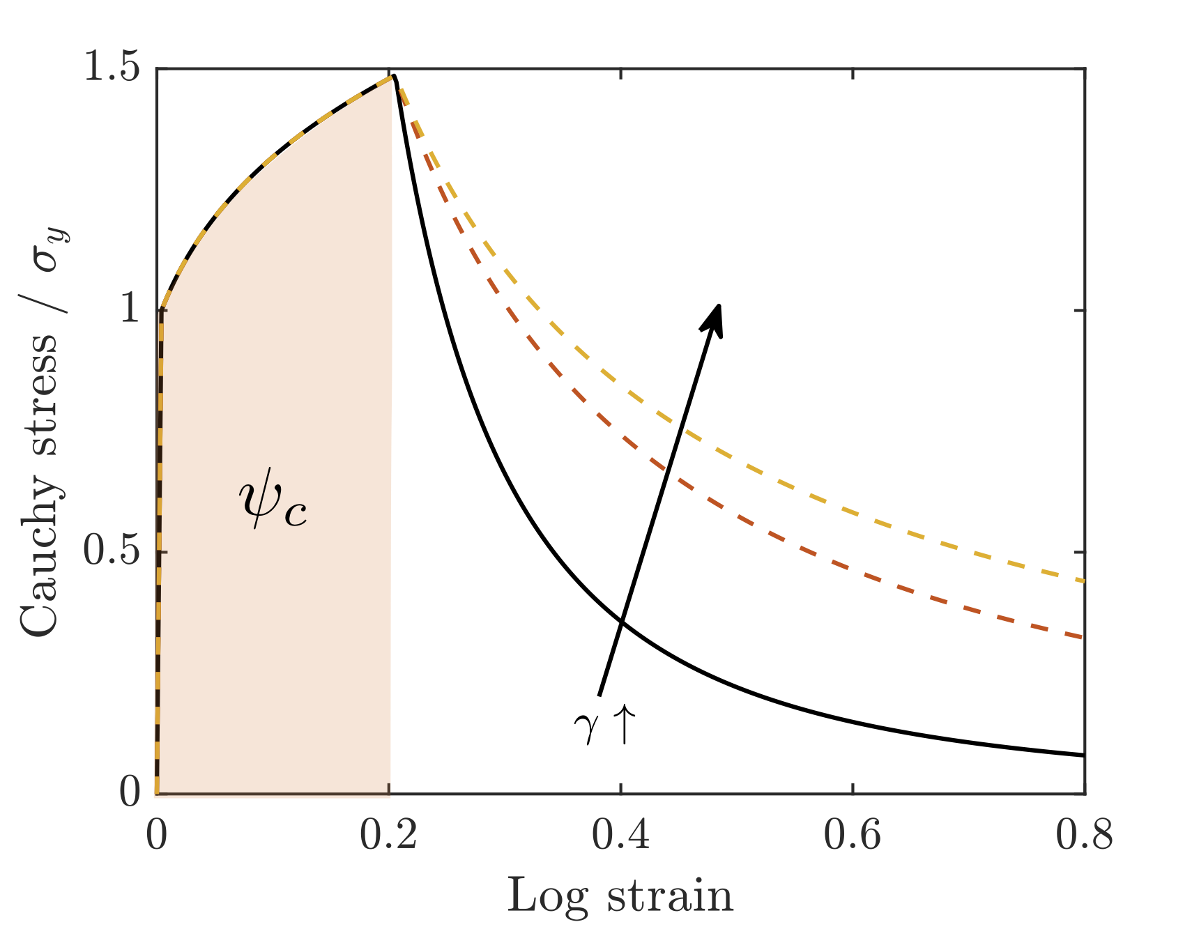
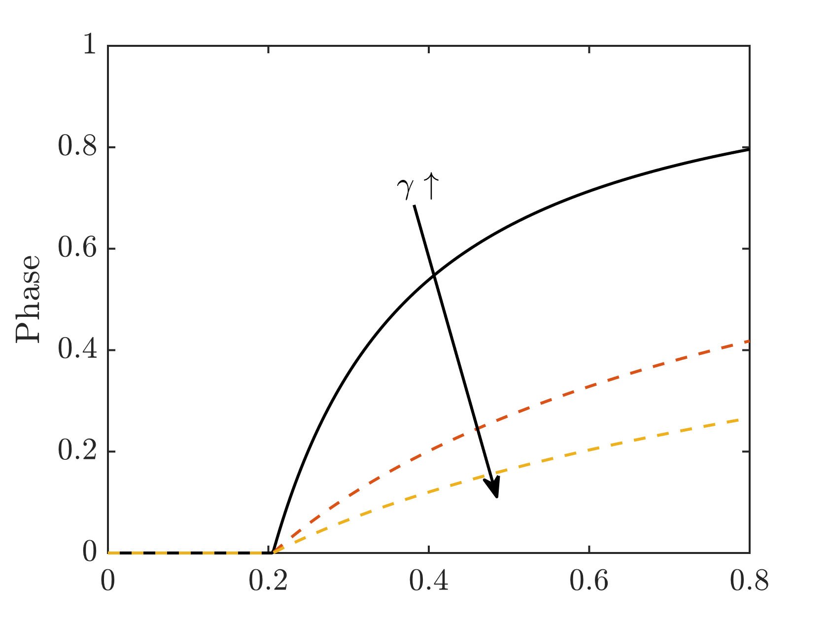
Fig. 4.156 Behavior of the model with the rational degradation function in homogeneous uniaxial tension. Data are shown for \(\gamma = \lbrace 0, 1, 2 \rbrace\). The solid lines are for \(\gamma = 0\). (a) Damage nucleates when the free energy density reaches the value of the model parameter \(\psi_c\), regardless of the value of \(\gamma\). The softening behavior is sensitive to \(\gamma\). (b) The rate of damage with strain decreases as \(\gamma\) increases.

The Lorentz degradation function is the only degradation function currently available in Phase Field F^eF^p, so \({g^e} = g^{\text{R}}\). The plastic degradation function is assumed to equal the elastic one, with an additional parameter \(p_{pl}\), which controls the portion of plastic work that contributes to driving fracture:

\[{g^p}(\phi) = (1-p_{pl}) + p_{pl} {g^e}(\phi) .\]

Many ductile phase-field references include the plastic work as driving energy (\(p_{pl}=1\), \({g^p}={g^e}\)), while others do not (\(p_{pl}=0\), \({g^p} = 1\)). This parameter allows for selection of either convention or an intermediate portion.

4.36.2.4. Tension-Compression Split

Two choices of tension-compression split have been implemented so far: none and volumetric-deviatoric. The none option includes all energy into the positive, damaging portion, holding nothing back in the negative portion:

\[\begin{split}\begin{cases} \widetilde{\psi}^e_+ = \widetilde{\psi}^e \\ \widetilde{\psi}^e_- = 0 \\ \psi^e(u,z,\phi) = {g^e}(\phi) \widetilde{\psi}^e(u,z) \\ \sigma^{M} = \frac{\partial \psi^e}{\partial {\varepsilon^{e}}} = {g^e}(\phi) \left( 2 \mu \mathrm{dev}({\varepsilon^{e}}) + \kappa \mathrm{tr}( {\varepsilon^{e}}) \right) \\ \psi^p(z,\phi) = {g^p}(\phi) \widetilde{\psi}^p(z) \end{cases} .\end{split}\]

The second option, volumetric-deviatoric, divides the elastic potential into volumetric and deviatoric components. The volumetric components contribute to the positive elastic potential only if the trace of the elastic strain tensor is positive (dilatational), while the deviatoric components always contribute. The plastic potential is not divided. The tension-compression split of the elastic potential also has implications for the definition of the stress:

\[\begin{split}\begin{cases} \widetilde{\psi}^e_+ = \frac{\kappa}{2} \left( \left< \mathrm{tr}( {\varepsilon^{e}}) \right>_+ \right)^2 + \mu \mathrm{dev}({\varepsilon^{e}}):\mathrm{dev}({\varepsilon^{e}}) \\ \widetilde{\psi}^e_- = \frac{\kappa}{2} \left( \left< \mathrm{tr}( {\varepsilon^{e}}) \right>_- \right)^2 \\ \psi^e(u,z,\phi) = {g^e}(\phi) \widetilde{\psi}^e_+(u,z) + \widetilde{\psi}^e_- \\ \sigma^{M} = \frac{\partial \psi^e}{\partial {\varepsilon^{e}}} = {g^e}(\phi) \left( 2 \mu \mathrm{dev}({\varepsilon^{e}}) + \kappa \left< \mathrm{tr}( {\varepsilon^{e}}) \right>_+ \right) + \kappa \left< \mathrm{tr}( {\varepsilon^{e}}) \right>_- \\ \psi^p(z,\phi) = {g^p}(\phi) \widetilde{\psi}^p(z) \end{cases} ,\end{split}\]

with Macaulay brackets indicating inclusion of positive \(\left< \cdot \right>_+\) or negative \(\left< \cdot \right>_-\) quantities.

A common third option, a spectral split that divides energy based on positive/negative eigenvalues of the strain tensor, has not been implemented to date.

4.36.3. Implementation

Implementational details of Phase Field F^eF^p is included in this section. This includes: (a) deviations between the theory and implementation, (b) an overview of the coupled solution strategy, (c) an overview of the solid mechanics solution, (d) an overview of the phase-field evolution solution.

4.36.3.1. Deviations from theory

4.36.3.1.1. Conditioning coefficient

For numerical stability reasons, the degradation function is implemented in the slightly modified form

(4.247)\[g(\phi) = g^{\text{R}}(\phi) (1 - k_c) + k_c,\]

where \(k_c \ll 1\) is a small, non-negative parameter called the conditioning coefficient that helps to avoid numerical problems such as element inversion in highly damaged material points. This modification directly impacts the stress and the driving energies \({g^e} \widetilde{\psi}^e_+ + {g^p} \widetilde{\psi}^p\); neither of these drop to zero as \(\phi\) approaches zero. This leaves a small residual stiffness in the material point to resist inversion, but with driving energies still active, the damage may continue to creep outward from fully-damaged areas. The use of conditioning coefficients is widespread throughout the phase-field fracture literature, e.g., [[10], [11], [12]]. Other techniques, such as removal of highly degraded elements using element death, could be used address this problem, though with a different set of tradeoffs.

4.36.3.1.2. Phase-field bound constraint

Examination of the phase-field update equation (4.237) in an unloaded state (i.e., {\(\widetilde{\psi}^e_+, \widetilde{\psi}^p\} = 0\)) with a uniform phase field (i.e., \(\Delta \phi = 0\)) reveals the need for an enforcement strategy for the phase field bound constraint \(\phi \leq 1\) in some formulations, such as the threshold model with the AT-1 damage potential (4.241).

The classical phase-field fracture model (AT-2, unimplemented) requires no constraint enforcement, as the solution to this case falls at the bound itself, \(\phi = 1\). In contrast, for the threshold model (AT-1, \({g^{\text{Q}}}\)), the update equation (4.239) simplifies to the following solution for a uniform state:

(4.248)\[\phi = \frac{3 G_c }{16 \ell \left( \widetilde{\psi}^e_+ + \widetilde{\psi}^p \right)}.\]

Clearly, when the driving energies are zero the solution of the phase field is infinite. For all values of \(\widetilde{\psi}^e_+ + \widetilde{\psi}^p\) less than the critical energy \(\frac{3 G_c }{16 \ell}\) will yield a phase field \(\phi > 1\), in violation of the phase bound. Enforcement of the phase field constraint is handled by employing a \(\max\)-function to enforce a sufficient driving energy that guarantees constraint satisfaction. We replace the usage of \(\widetilde{\psi}^e_+ + \widetilde{\psi}^p\) with \(\psi^D_+\), defined as:

(4.249)\[\psi^D_+ = \max \left( \widetilde{\psi}^e_+ + \widetilde{\psi}^p, \frac{3 G_c }{16 \ell} \right)\]

Generalizing this for the rational degradation function \(g^{\text{R}}(\phi)\) in the cohesive phase field model yields (derivation omitted):

(4.250)\[\psi^D_+ = \max \left( \widetilde{\psi}^e_+ + \widetilde{\psi}^p, \psi_c \right) = \langle \widetilde{\psi}^e_+ + \widetilde{\psi}^p - \psi_c \rangle + \psi_c ,\]

where \(\langle \bullet \rangle\) are Macaulay brackets.

This boundary treatment is derived from the homogeneous case (\(\phi=1\)); for a phase field that is not spatially uniform, there may be small violations. This approximation is widely used in the literature (e.g., Miehe [[11]]) and thought to be a reasonable approximation.

While this approach ordinarily provides for satisfaction of the phase-field bound constraint, we note that it does affect the physics of the problem. The resulting phase-field solutions and energy dissipation may differ from analytical solutions that enforce the bound constraint differently.

4.36.3.1.3. Phase-field irreversibility constraint

A longstanding strategy for addressing the phase-field irreversibility constraint is to modify the fracture driving energies through the use of a history function, as proposed by Miehe et al. [[13]]:

\[\mathcal{H}(x,t) = \max_{\hat{t} \in [0, t]} \psi^D_+(x,\hat{t}) .\]

Practically, this can be enforced by maintaining the history-maximum driving energy as a state variable on the integration points and comparing at each time step:

\[\mathcal{H}(x,t_{n+1}) = \max \left( \psi^D_+(x,t_{n+1}), \mathcal{H}(x,t_n) \right) .\]

The monotonicity of the phase-field driving force approximately enforces irreversibility. Together with the bound-constraint modification, the phase-field update equation (formerly (4.237)) now reads:

(4.251)\[\frac{\partial \psi^f}{\partial \nabla{\phi}} G_c - \frac{\partial {g^e}(\phi)}{\partial \phi} \mathcal{H} - \frac{\partial \psi^f}{\partial \phi} G_c = 0.\]

For the implemented damage potential implemented (AT-1), this becomes:

(4.252)\[\frac{3 G_c \ell}{4} \Delta \phi - \frac{\partial {g^e}(\phi)}{\partial \phi} \mathcal{H} + \frac{3 G_c}{8 \ell} = 0 .\]

Geelen et al. [[14]] explored the use of an augmented-Lagrangian formulation as an alternative means of enforcing the bound and irreversibility constraints. Their finding was that the history function causes slight increases in global energy dissipation, corresponding to widening of the damage fields around cracks. The additional cost of the augmented-Lagrangian formulation, both in implementation and operation, has been a barrier to its implementation in Sierra so far.

4.36.3.2. Coupled solution strategy for implicit time integration

In order to solve the Euler-Lagrange equations (4.234) for the phase-field fracture model, an alternating minimization strategy is employed. In this approach, the conventional balance-of-linear-momentum boundary-value problem is solved in terms of its displacement degrees of freedom, with a return-mapping algorithm for the plastic state variables and the phase field held constant. The phase-field Euler-Lagrange equation (4.237) is then solved with the inputs from the displacement system (driving energies) held constant. Equilibrium between the two fields is achieved by solving the two subproblems repeatedly in a staggered fashion until convergence in both fields is observed. This procedure is illustrated in Fig. 4.157.

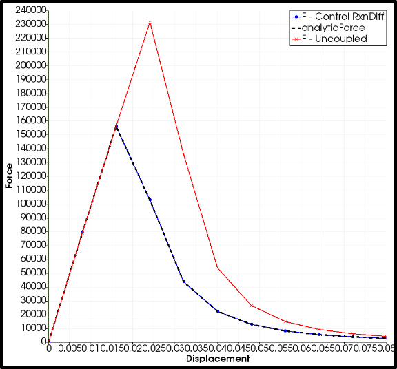
Fig. 4.157 Alternating minimization scheme behavior. (a) Schematic of alternating minimization scheme. At a new time step \(t_{n+1}\), nonlinear solves for mechanics (M) and phase field (PF) are repeated until convergence achieved in both fields. Solver then proceeds to the next time step. (b) Force vs. displacement for a single element uniaxial tension problem with elastic material. The exact solution for the problem is shown with a dotted line. the curve marked “uncoupled” is solved with a single pass at each time step, leading to a solution that is out of equilibrium. The curve “ControlRxnDiff” is solved until convergence, indicating equilibrium. The equilibrium result is seen to agree with the exact solution.

This approach is selected primarily due to its consistency with Sierra paradigm for multi-field problems and therefore ease of implementation. Building within the framework of Sierra/SM, it is expedient to leave the traditional displacement system solution as-is, modified only by a damage term relating to the phase-field. This approach is very commonly used in the phase field literature (see, e.g., [[10], [13]]). Solution of each sub-problem is straightforward, as each is convex; however, with the cross-terms held fixed, the alternating coupled solve may be slow to converge at times.

The alternative approach is a monolithic solve, wherein the coupled displacement-phase system is solved as a single matrix system. This approach has been used by several authors (e.g., [[14], [9], [3]]), and exhibits improved convergence in some cases; however, the solution may stall at saddle points as the convexity of the coupled system is not guaranteed. Monolithic solution is not implemented in Sierra/SM.

4.36.4. Operator split scheme for explicit time integration

The algorithm for explicit integration is a straightforward extension of the quasi-static scheme outlined above. The major difference is that there is no equilibrium iteration between the fields on a given time step. Iteration is unnecessary given the small size of the time steps dictated by the numerical stability condition. Another consequence of the small time-step size is that the phase field need not be updated at each time step. (An exception to this may be if the loading conditions are in the shock regime.) The phase-field balance equation is also nonlinear, incurring a greater computational cost than an explicit time integration step, and it is therefore desirable to amortize this cost over a number of time steps. The frequency of the phase field update has been made a user-defined choice in the input file.

4.36.4.1. Solid mechanics solution

The full derivation of the solid mechanics solution is provided in the cited references [[1], [2], [3]]. The return mapping algorithm for the Phase Field F^eF^p constitutive update, which corresponds to the solution of the state-variable Euler-Lagrange equation (4.236) will be specifically described in this section.

The Phase Field F^eF^p uses a radial return predictor-corrector algorithm for the constitutive update. First, an elastic trial stress state is calculated. This is done by assuming that the deformation increment is completely elastic and that the phase field has remained constant:

\[\begin{split}\begin{cases} {F^{p, tr}} &= {F^p}_{n} \\ \bar{\varepsilon}^{p,tr} &= \bar{\varepsilon}^p_{n} \\ {F^{e, tr}} &= F_{n+1} {F^{p, tr}}^{-1} \\ \phi_{n+1} &= \phi_{n} \end{cases} .\end{split}\]

The trial deformation state is converted to logarithmic strains to compute a conjugate Mandel trial stress (the trial Mandel stress shall be consistent with the tension-compression split, defined in Section 4.36.2.4. The baseline (no tension-compression case) is given here):

\[{C^{e, tr}} = {F^{e, tr}}^T {F^{e, tr}} ,\]

\[{\varepsilon^{e, tr}} = \frac12 \log({C^{e, tr}}),\]

\[\sigma^{M,tr} = {g^e}(\phi_{n+1}) \left( 2 \mu \mathrm{dev}({\varepsilon^{e, tr}}) + \kappa \mathrm{tr}( {\varepsilon^{e, tr}}) \right)\]

An effective stress is calculated:

\[\bar{\sigma}^{tr} = \sqrt{\frac{3}{2}} ||\mathrm{dev}{\sigma^{M,tr}}|| ,\]

and compared to the flow stress, determined by evaluating the hardening model with the trial plastic strain scalar \(\bar{\varepsilon}^{p,tr}\) and factoring by the plastic degradation function \({g^p}\):

\[\bar{Y}^{\mathrm{eq},tr} = {g^p}(\phi_{n+1}) Y^{\mathrm{eq}}(\bar{\varepsilon}^{p,tr}) .\]

If \(\bar{\sigma}^{tr} \leq \bar{Y}^{\mathrm{eq},tr}\), then the deformation increment is elastic, and the stress update is finished: \(\sigma^m_{n+1} = \sigma^{M,tr}\), \(\Delta\bar{\varepsilon}^p=0\). If instead \(\bar{\sigma}^{tr} > \bar{Y}^{\mathrm{eq},tr}\), then plastic deformation had occurred and a radial return algorithm determines the extent of plastic deformation.

The normal to the yield surface is assumed to lie in the direction of the trial stress state. This gives the following expression for the flow tensor \(N^p_{n+1}\), with isotropic hardening assumed:

\[N^p_{n+1} = \sqrt{\frac{3}{2}} \frac{\sigma^{M,tr}}{||\sigma^{M,tr}||} = \frac{3}{2} \frac{\mathrm{dev}\,\sigma^{M,tr}}{\bar{\sigma}^{tr}}.\]

The radial return algorithm seeks to solve the following equation (The first two terms represent the new effective stress \(\bar{\sigma}(\varepsilon^e_{n+1})\) evaluated at \(\varepsilon^e_{n+1} = \varepsilon^{e, tr} - \Delta\bar{\varepsilon}^p N^p_{n+1}\). This corresponds to \(\frac{\partial\widetilde{\psi}^e_+}{\partial\bar{\varepsilon}^p} = \frac{\partial\widetilde{\psi}^e_+}{\partial\varepsilon^e}-N^p_{n+1}\). The last term represents the new flow stress \(Y^\mathrm{eq}(\bar{\varepsilon}^p_{n+1})\) evaluated at \(\bar{\varepsilon}^p_{n+1} = \bar{\varepsilon}^p_n + \Delta\bar{\varepsilon}^p\).):

\[\bar{\sigma} - 3\mu {g^e}(\phi_{n+1}) \Delta\bar{\varepsilon}^p - {g^p}(\phi_{n+1}) Y^{\mathrm{eq}}(\bar{\varepsilon}^p_{n} + \Delta\bar{\varepsilon}^p) = 0\]

using a Newton-Raphson algorithm, with residual \(\bar{R}\) and iteration denoted by superscript \(k\):

\[\begin{split}\begin{cases} \bar{R} &= \bar{\sigma} - 3\mu {g^e}(\phi_{n+1}) \Delta\bar{\varepsilon}^p - {g^p}(\phi_{n+1}) Y^{\mathrm{eq}}(\bar{\varepsilon}^p_{n} + \Delta\bar{\varepsilon}^p) \\ \frac{\partial \bar{R}}{\partial \Delta\bar{\varepsilon}^p} & = -3\mu {g^e}(\phi_{n+1}) - {g^p}(\phi_{n+1}) \frac{\partial Y^{\mathrm{eq}}}{\partial \Delta\bar{\varepsilon}^p}\/(\bar{\varepsilon}^p_{n} + \Delta\bar{\varepsilon}^p) \\ (\Delta\bar{\varepsilon}^p)^{k} &= 0 \\ (\Delta\bar{\varepsilon}^p)^{k+1} &= (\Delta\bar{\varepsilon}^p)^{k} -\bar{R} / \frac{\partial \bar{R}}{\partial \Delta\bar{\varepsilon}^p} \end{cases} .\end{split}\]

This equation is iterated until convergence, with a line search algorithm to accelerate convergence. The value \((\Delta\bar{\varepsilon}^p)^{k+1}\) that satisfies the convergence tolerance establishes the solution at time \(t_{n+1}\): \(\Delta\bar{\varepsilon}^p_{n+1} = (\Delta\bar{\varepsilon}^p)^{k+1}\). After the plastic update has been solved, the material state fields are updated (the updated Mandel stress shall be consistent with the tension-compression split, defined in Section 4.36.2.4. The baseline (no tension-compression case) is given here):

\[\begin{split}\begin{cases} \bar{\varepsilon}^p_{n+1} &= \bar{\varepsilon}^p_{n} + \Delta\bar{\varepsilon}^p_{n+1} \\ {F^p}_{n+1} &= \exp(\Delta\bar{\varepsilon}^p_{n+1} N^p_{n+1}) {F^p}_{n} \\ {F^e}_{n+1} &= F_{n+1} {F^p}_{n+1}^{-1} = {F^{e, tr}} \exp(-\Delta\bar{\varepsilon}^p_{n+1} N^p_{n+1}) \\ C^e_{n+1} &= {F^e}_{n+1}^T {F^e}_{n+1} = {C^{e, tr}} \exp(-2 \Delta\bar{\varepsilon}^p_{n+1} N^p_{n+1}) \\ {\varepsilon^{e}}_{n+1} &= {\varepsilon^{e, tr}} - \Delta\bar{\varepsilon}^p N^p_{n+1} \\ \sigma^m_{n+1} &= {g^e}(\phi_{n+1}) \left( 2 \mu \mathrm{dev}({\varepsilon^{e}}_{n+1} ) + \kappa \mathrm{tr}( {\varepsilon^{e}}_{n+1} ) \right) \\ \bar{\sigma}_{n+1} &= \bar{\sigma}^{tr} - 3\mu {g^e}(\phi_{n+1}) \Delta\bar{\varepsilon}^p_{n+1} \\ \sigma_{n+1} &= \frac{1}{||F_{n+1}||} {F^e}_{n+1}^{-T} \sigma^m_{n+1} {F^e}^{T} \end{cases} .\end{split}\]

These fields are then used to calculate the driving energies \(\{\widetilde{\psi}^e_+,\widetilde{\psi}^p\}\) for the phase-field update solve. The elastic potential is calculated using \({F^e}_{n+1}\), as defined in Section 4.36.1.2; the plastic potential is calculated using \(\bar{\varepsilon}^p_{n+1}\), as defined in Section 4.36.2; the final driving energies are created using these potentials, modified by the tension-compression split (Section 4.36.2.4) and the bound-constraint and irreversibility treatments (Section 4.36.3.1).

4.36.4.2. Phase-field evolution solution

The phase-field update equation (4.252) is solved in Sierra/SM’s reaction-diffusion solver, using a Galerkin finite element approach to solve the equation in weak form. The same finite element mesh is used for both the displacement solve and the phase-field solve (an alternative solution method is to use Arpeggio to couple with Aria’s reaction-diffusion solution capability. Due to the complexity of the input file and the need to compile a custom user-plugin for the source term, this is not recommended. This approach does, however, allow for a different mesh to be used for the phase-field solve).

The weak form is derived by first taking the inner product of the phase-field update equation with a phase variation \(\omega\) over the domain \(\Omega\):

\[\int_{\Omega} \frac{3 G_c \ell}{4} \Delta \phi \omega - \frac{\partial {g^e}(\phi)}{\partial \phi} \mathcal{H} \omega + \frac{3 G_c}{8 \ell} \omega \,d\Omega= 0 .\]

We linearize the degradation function term \(\frac{\partial {g^e}(\phi)}{\partial \phi} \rightarrow \frac{\partial^2 {g^e}(\phi)}{\partial \phi^2} \phi\) in order to accommodate the rational degradation function \(g^{\text{R}}\), and then integrate by parts and rearrange to achieve a bilinear form:

\[\int_{\Omega} \frac{3 G_c \ell}{4} \nabla{\phi} \cdot \nabla{\omega} + \frac{\partial^2 {g^e}(\phi)}{\partial \phi^2} \mathcal{H} \phi \omega \,d\Omega = \int_{\Omega} \frac{3 G_c}{8 \ell} \omega \,d\Omega + \int_{\partial\Omega} \frac{3 G_c \ell}{4} \nabla{\phi} \omega \cdot {n}_{\partial\Omega} \,d\Gamma .\]

The last term can be omitted as the variation \(\omega=0\) is defined to be zero on the boundary. The phase field and phase variation are discretized using the existing mesh shape functions \(N_i\):

\[\begin{split}\begin{cases} \phi &= \sum_i N^A_i(x) \phi_i \\ \nabla{\phi} &= \sum_i \nabla{N^A_i}(x) \phi_i \\ \omega &= \sum_j N^B_j(x) \omega_j \\ \nabla{\omega} &= \sum_j \nabla{N^B_j}(x) \omega_j \end{cases} ,\end{split}\]

\[\sum_{\{i,j\}} \left(\int_{\Omega} \frac{3 G_c \ell}{4} \nabla{N^A_i}(x) \phi_i \cdot \nabla{N^B_j}(x) \omega_j + \frac{\partial^2 {g^e}(\phi)}{\partial \phi^2} \mathcal{H} N^A_i(x) \phi_i N^B_j(x) \omega_j \,d\Omega = \int_{\Omega} \frac{3 G_c}{8 \ell} N^B_j(x) \omega_j \,d\Omega \right) .\]

The phase variation nodal field \(\omega_j\) can then be factored out:

\[\sum_{\{i,j\}} \left(\phi_i\int_{\Omega} \frac{3 G_c \ell}{4} \nabla{N^A_i}(x) \cdot \nabla{N^B_j}(x) + \frac{\partial^2 {g^e}(\phi)}{\partial \phi^2} \mathcal{H} N^A_i(x) N^B_j(x) \,d\Omega = \int_{\Omega} \frac{3 G_c}{8 \ell} N^B_j(x) \,d\Omega \right).\]

Gaussian quadrature is used in each element to compute the shape function integrals and then the element systems are assembled into the global system. In the spirit of the reaction-diffusion equation template, we refer to the first term as the diffusion term \(D_{ij}=\frac{3 G_c \ell}{4} \nabla{N^A_i} \cdot \nabla{N^B_j}\), the second as the reaction term \(R_{ij}=\frac{\partial^2 {g^e}(\phi)}{\partial \phi^2} \mathcal{H} N^A_i N^B_j\), and the right-hand side as the source term \(S_j= \frac{3 G_c}{8 \ell} N^B_j\). We note that the diffusion term has the form of a stiffness matrix, while the reaction term has the form of a mass matrix. The system of equations can then be restated as:

\[\left(D_{ij} + R_{ij} \right) \phi_i = S_j .\]

In fact, the phase-field update is solved incrementally; that is to say that we solve for \(\Delta \phi\), rather than \(\phi_{n+1} = \phi_{n} + \Delta \phi\) directly. This updates the matrix system to be written as:

\[\left(D_{ij} + R_{ij} \right) (\phi_{n} + \Delta \phi)_i = S_j .\]

Further, we note that the system of equations is linear for the quadratic degradation function \({g^{\text{Q}}}\) as \(\frac{\partial^2 {g^{\text{Q}}}(\phi)}{\partial \phi^2}=2\), but is generally nonlinear for the rational degradation function \(g^{\text{R}}\), with \(R=R(\phi)\). For linear systems (\({g^e} = {g^{\text{Q}}} = g^{\text{R}}(\gamma=0)\)), we solve the system for \(\Delta \phi\) directly, as:

(4.253)\[\left(D_{ij} + R_{ij} \right) (\Delta \phi)_i = S_j - \left(D_{ij} + R_{ij} \right) (\phi_{n})_i .\]

For nonlinear systems (\({g^e} = g^{\text{R}}(\gamma \ne 0)\)), the phase-field increment is solved using an iterative preconditioned conjugate gradient solver that minimizes the residual of (4.253). The nodal preconditioner is established using a probing approach.

4.36.4.2.1. Bound constrained solve

While the approaches described in Section 4.36.3.1 tend to enforce the phase field bound and irreversibility constraints fairly well, in practice, there are situations in which they occasionally fail. Assuming that the phase field is properly initialized, the upper bound (\(\phi \leq 1\)) will be respected as long as the irreversibility constraint \(\Delta \phi \leq 0\) is met. This leaves the irreversibility constraint and the lower bound (\(\phi \geq 0\)) as the relevant bounds.

The phase-field solve is augmented with bound-constraint methods in order to ensure that the constraints are satisfied. For the linear solve, this is implemented by simply restricting the phase field to bounds: \(0 \leq \phi_{n+1} \leq \phi_{n}\) ; violating values are set to the bound. Further, for the nonlinear solve with conjugate gradient, the conjugate-gradient step size is set to zero at nodes where the bound constraint is active. Details of this algorithm can be found in Vollebregt [[15]].

While this approach appears to do an adequate job at satisfying the bound constraints on the phase field, we retain the driving energy modifications defined in Section 4.36.3.1 until it is demonstrated that the bound-constrained conjugate gradient solve successfully reproduces known solutions.

4.36.5. Verification

Both single-material point unit tests and full regression tests are used to verify the Phase Field F^eF^p model.

4.36.5.1. Unit testing

The Phase Field F^eF^p model is verified through a series of uniaxial stress test considering a variety of load magnitudes and phase-field model forms, loosely based on the boundary value problems of Appendix A are used. Throughout these tests, the elastic properties are maintained as \(E=200\) GPa and \(\nu = 0.3\), the plasticity is defined as linear hardening with \({Y_0}=180\) MPa and \(H=180\) MPa, the fracture parameters are set to \(G_c=6.2\) J/m \(^2\), \(\ell=1.34`m, :math:`k_c = 1.2\cdot 10^{-4}\), \(p_{pl}=1\) , and a phase field of \(\phi=0.9\). The phase-field model is tested with both the threshold (AT-1) model (\(\gamma=0\), \(\psi_c=\frac{3}{16}\frac{G_c}{\ell}\)) and the Lorentz model (\(\gamma=2\), \(\psi_c=\frac{1}{16}\frac{G_c}{\ell}\)) and with the two implemented tension-compression splits (none and volumetric-deviatoric). For these tests, we compare the Cauchy stress (often in the uniaxial component) and plastic strain \(\bar{\varepsilon}^p\) as well as the fracture and driving energies.

4.36.5.1.1. Uniaxial Tension - Elastic

For this problem, we set the following deformation state, with the applied axial strain to be half of the yield strain to ensure elasticity:

\[\begin{split}\begin{cases} \varepsilon_{11} &= \frac12 \frac{{Y_0}}{E} \\ \varepsilon_{22} = \varepsilon_{33} &= -\nu \varepsilon_{11} \\ F_{11} &= \exp(\varepsilon_{11}) \\ F_{22} = F_{33} &= \exp(\varepsilon_{22}) = \exp(-\nu \varepsilon_{11}) \\ \nabla{\phi} \cdot \nabla{\phi} &= 0 \end{cases}\end{split}\]

This is equivalent to \(\lambda = \exp(\frac12 \frac{{Y_0}}{E}) - 1\). Analytical solutions for the stress, plastic strain, and energies are derived for comparison. The phase-field models considered are the threshold (AT-1) and Lorentz degradation functions. The tension-compression split is not tested as it would not be active in this case. %Begin elastic, the expected stress is \(\sigma = \frac{E \varepsilon_{11}}{\exp((1-2\nu) E \varepsilon_{11})} \mathrm{deg}(\phi)\), the plastic strain is \(\bar{\varepsilon}^p=0\)

4.36.5.1.2. Uniaxial Tension - Plastic

For this problem, we set the following deformation and phase state, with the applied axial strain to be 150% of the yield strain to ensure plasticity:

\[\begin{split}\begin{cases} \varepsilon_{11} &= \frac32 \frac{{Y_0}}{E} \\ \varepsilon_{22} = \varepsilon_{33} &= -\nu \varepsilon_{11} \\ F_{11} &= \exp(\varepsilon_{11}) \\ F_{22} = F_{33} &= \exp(\varepsilon_{22}) = \exp(-\nu \varepsilon_{11}) \\ \nabla{\phi} \cdot \nabla{\phi} &= 0.1 \end{cases}\end{split}\]

Analytical solutions for the stress, plastic strain, and energies are derived for comparison. The phase-field models considered are the threshold (AT-1) and Lorentz degradation functions. Additionally, the plastic-work driving energy portion parameter \(p_{pl}\) is tested at additional values of \(p_{pl} = \{0, 0.5\}\) . The tension-compression split is not tested as it would not be active in this case.

4.36.5.1.3. Uniaxial Compression - Elastic

For this problem, we set the following deformation and phase state, with the applied axial strain to be negative half of the yield strain to ensure elasticity:

\[\begin{split}\begin{cases} \varepsilon_{11} &= -\frac12 \frac{{Y_0}}{E} \\ \varepsilon_{22} = \varepsilon_{33} &= -\nu \varepsilon_{11} \\ F_{11} &= \exp(\varepsilon_{11}) \\ F_{22} = F_{33} &= \exp(\varepsilon_{22}) = \exp(-\nu \varepsilon_{11}) \\ \nabla{\phi} \cdot \nabla{\phi} &= 0 \end{cases}\end{split}\]

Analytical solutions for the stress, plastic strain, and energies are derived for comparison. The phase-field models considered are a matrix of degradation functions (threshold and Lorentz) and the tension-compression splits (none and volumetric-deviatoric).

4.36.5.2. Regression testing

Several tests are implemented in Sierra/SM’s regression test library to provide regular testing of the Phase Field F^eF^p in a full finite-element setting. While some of the tests have no analytical solution and are simply compared to an accepted “gold” result file, others include solution verification to known analytical solutions. At a minimum, the former tests include solution verification of the phase bound constraints when the bound-constrained solver is applied.

The tests with solution verification are detailed here:

4.36.5.2.1. 1D PhaseBC FeFp

% with dimensions \(x\in [-0.05,0.05]\), \(y\in [-0.0005,0.0005]\), \(z\in [-0.0005,0.0005]\) In this test, a 1-D bar is subjected to a Dirichlet phase boundary condition \(\phi=0\) at the center \(x=0\), representing an initial crack. Displacement is fixed on the entire domain, and the nonlinear reaction-diffusion solver solves for the phase-field emanating from the center. This test checks the phase profile against an analytical solution (4.254) both as mesh is refined (successively tighter tolerances) and as Lorentz degradation parameter \(\gamma\) is varied (\(\gamma = 0\) and \(\gamma \rightarrow \infty\)). This is critical as single-material-point unit tests cannot verify a spatial phase-field solution.

With no mechanical work, the driving energy relies on the critical energy threshold to satisfy the phase boundary condition: \(\mathcal{H} = \psi_c\). Adapting (4.252) for this case reads:

\[\frac{3 G_c \ell}{4} \phi_{,xx} - \frac{2\phi(1+\gamma)}{(1+\gamma - \phi\gamma)^3} \frac{3 G_c}{16 \ell (1+\gamma)} + \frac{3 G_c}{8 \ell} = 0\]

subject to

\[\begin{split}\begin{cases} 0 \leq \phi \leq 1 \\ \phi(0)=0 \\ \phi(x_0) = 1 \\ \phi_{,x}(x_0) = 0 \end{cases} .\end{split}\]

The analytical solution for the cases above is:

(4.254)\[\begin{split}\phi(x) = \begin{cases} 1 - \exp(-\frac{|x|}{\sqrt{2\ell}}) \mbox{ with } x_0 = \infty & \mbox{for } \gamma = 0 \\ 1 - \left(1 - \frac{|x|}{2\ell} \right)^2 \mbox{ with } x_0 = 2\ell & \mbox{for } \gamma \rightarrow \infty \end{cases} .\end{split}\]

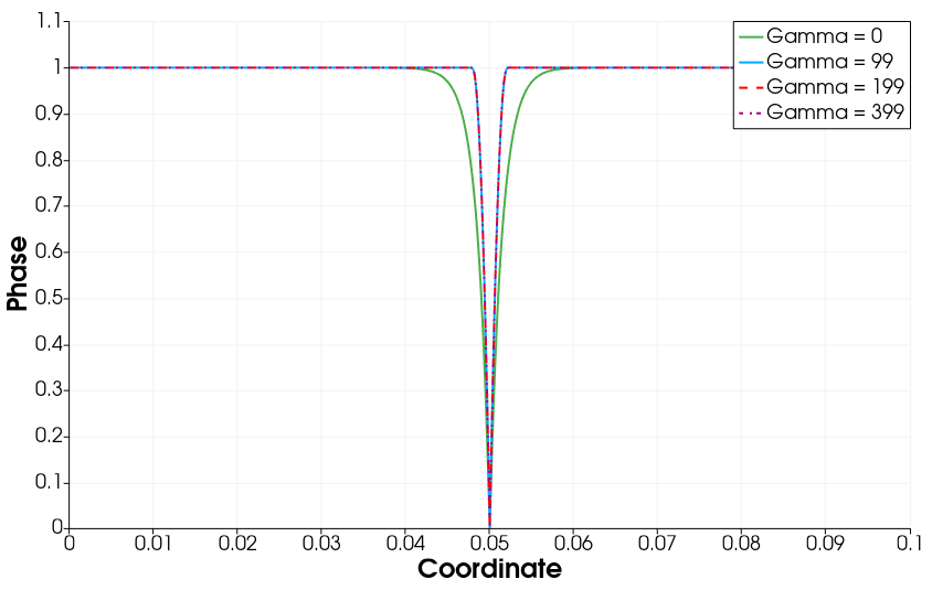
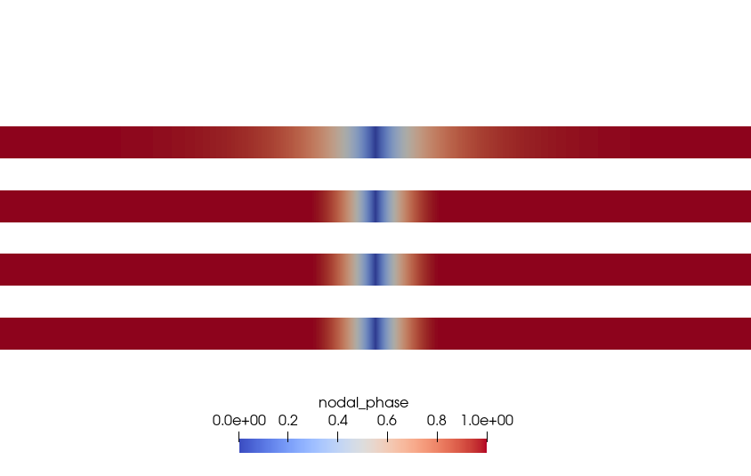
Fig. 4.158 Imagery showing the phase field solutions generated from the 1D PhaseBC FeFp verification test, with the phase boundary condition placed at \(x=0.5\) and \(\ell = 0.001\).

4.36.5.2.2. Control 1-D Extension

In this test, a cube is pulled in uniaxial tension with a displacement boundary condition through the elastic, plastic, and damage regimes. The phase-field length scale \(\ell\) is set to be very large compared to the domain, so that the phase-field solution remains uniform and the gradient terms are negligible. The phase-field model form is set to the threshold (AT-1) model with \(\gamma = 0\), and the linear reaction diffusion solver is used. The test checks against the reaction force required to assert the boundary condition as well as the phase-field in the body. Both linear-elastic and elastic-plastic materials are considered, each at a single-element and multiple-element mesh.

The analytical solution for the linear-elastic case is

(4.255)\[\begin{split}\begin{cases} \varepsilon _{11}&= \log(1 + u/L) \\ \varepsilon^e _{11} &= \varepsilon_{11} \\ \widetilde{\psi}^e &= \frac12 E (\varepsilon^e_{11})^2 \\ \phi &= \min(1, \psi_c/\widetilde{\psi}^e) \\ P &= \phi^2 \frac{ E \varepsilon^e_{11}}{\exp(\varepsilon^e_{11})} \\ f &= P A_0 \end{cases} ,\end{split}\]

while the analytical solution for the elastic-plastic case is

(4.256)\[\begin{split}\begin{cases} \varepsilon _{11} &= \log(1 + u/L) \\ \varepsilon^e _{11} &= \min( \varepsilon_{11}, \frac{H \varepsilon_{11} + {Y_0}}{H E} ) \\ \varepsilon^p _{11} &= \varepsilon _{11} - \varepsilon^e _{11}\\ \bar{\varepsilon}^p &= \varepsilon^e_{11} \\ \widetilde{\psi}^e &= \frac12 E (\varepsilon^e_{11})^2 \\ \widetilde{\psi}^p &= \frac12 H (\bar{\varepsilon}^p)^2 + {Y_0} \bar{\varepsilon}^p \\ \phi &= \min(1, \psi_c/(\widetilde{\psi}^e+\widetilde{\psi}^p) ) \\ P &= \phi^2 \frac{ E \varepsilon^e_{11}}{\exp(\varepsilon^e_{11})} \\ f &= P A_0 \end{cases} ,\end{split}\]

where \(P\) is the first Piola-Kirchhoff stress, \(A_0\) represents the initial cross-sectional area, \(u\) represents axial displacement, \(L\) represents the initial length of the cube, \(f\) represents the reaction force, and \(H\) represents the linear hardening slope. The test checks against the reaction force required to assert the boundary condition as well as the phase-field in the body.

4.36.5.2.3. Single Element, Linear

This test reproduces a specific case of the Control 1-D Extension test (linear-elastic, single element), but adds consideration of the conditioning coefficient \(k_c\). The phase-field model form is set to the threshold (AT-1) model with \(\gamma = 0\), and the linear reaction-diffusion solver is used. The test checks against the reaction force required to assert the boundary condition as well as the phase-field in the body.

The analytical solution is

(4.257)\[\begin{split}\begin{cases} \varepsilon _{11}&= \log(1 + u/L) \\ \varepsilon^e _{11} &= \varepsilon_{11} \\ \widetilde{\psi}^e &= \frac12 E (\varepsilon^e_{11})^2 \\ \phi &= \min \left(1, \frac{\psi_c}{\widetilde{\psi}^e (1-k_c)+\psi_c k_c} \right) \\ P &= (\phi^2 (1-k_c) + k_c) \frac{ E \varepsilon^e_{11}}{\exp(\varepsilon^e_{11})} \\ f &= P A_0 \end{cases} .\end{split}\]

4.36.5.2.4. Single Element, Nonlinear as Linear

This test reproduces a specific case of the Control 1-D Extension test (linear-elastic, single element), but adds consideration of the nonlinear reaction diffusion solver. The phase-field model form is set to the threshold (AT-1) model with \(\gamma = 0\), but the nonlinear reaction-diffusion solver is used. Additionally, the impact of the tension-compression split is verified by loading in uniaxial tension (no split, volumetric-deviatoric split) and uniaxial compression (no split). The solution for the volumetric-deviatoric split in uniaxial compression is skipped due to its complex derivation, though it is verified numerically in the next test. The test checks against the reaction force required to assert the boundary condition as well as the phase-field in the body. Together with Single Element, Linear, this test verifies that the linear and nonlinear reaction-diffusion solvers provide the same result for the linear \(\gamma=0\) case.

4.36.5.2.5. Single Element, Nonlinear

This test reproduces a specific case of the Control 1-D Extension test (linear-elastic, single element), but adds consideration of the nonlinear reaction diffusion solver. The phase-field model form is set to the Lorentz model with \(\gamma = 0.48\). Additionally, the impact of the tension-compression split is verified by loading in uniaxial tension and uniaxial compression, while applying both no split and the volumetric-deviatoric split for each. The test checks against the reaction force required to assert the boundary condition as well as the phase-field in the body. The derivation of a closed-form complex, so a comparison solution has been prepared using symbolic and numerical solution in a Matlab script solve_Lorentz.m.

4.36.6. User Guide

BEGIN PARAMETERS FOR MODEL PHASE_FIELD_FEFP
  #
  # Elastic constants
  #
  YOUNGS MODULUS = <real>
  POISSONS RATIO = <real>
  SHEAR MODULUS  = <real>
  BULK MODULUS   = <real>
  LAMBDA         = <real>
  TWO MU         = <real>
  #
  # Phase Field parameters
  #
  CONDITIONING COEFFICIENT            = <real>
  CRITICAL ENERGY DENSITY             = <real> (3.0/16.0 * GC / FLS)
  FRACTURE LENGTH SCALE               = <real>
  GC                                  = <real>
  NONLOCAL SOLVER                     = NONE | ARIA | RXNDIFF (RXNDIFF)
  PLASTIC WORK DRIVING ENERGY PORTION = <real> (1.0)
  TENSION COMPRESSION SPLIT           = VOLUMETRIC_DEVIATORIC | NONE (NONE)
  #
  # Yield surface parameters
  #
  YIELD STRESS = <real>

#
  #
  # Hardening model
  #
  HARDENING MODEL = LINEAR | POWER_LAW | VOCE | USER_DEFINED |
  FLOW_STRESS | DECOUPLED_FLOW_STRESS | JOHNSON_COOK |
  POWER_LAW_BREAKDOWN
  #
  # Linear hardening
  #
  HARDENING MODULUS = <real>
  #
  # Power-law hardening
  #
  HARDENING CONSTANT = <real>
  HARDENING EXPONENT = <real> (0.5)
  LUDERS STRAIN      = <real> (0.0)
  #
  # Voce hardening
  #
  HARDENING MODULUS       = <real>
  EXPONENTIAL COEFFICIENT = <real>
  #
  # Johnson-Cook hardening
  #
  HARDENING FUNCTION = <string>hardening_function_name
  RATE CONSTANT      = <real>
  REFERENCE RATE     = <real>
  #
  # Power law breakdown hardening
  #
  HARDENING FUNCTION = <string>hardening_function_name
  RATE COEFFICIENT   = <real>
  RATE EXPONENT      = <real>
  # User defined hardening
  #
  HARDENING FUNCTION = <string>hardening_function_name
  #

#
  #
  # Following Commands Pertain to Flow_Stress Hardening Model
  #
  #    -  Isotropic Hardening model
  #
  ISOTROPIC HARDENING MODEL = LINEAR | POWER_LAW | VOCE |
                              USER_DEFINED
  #
  # Specifications for Linear, Power-law, and Voce same as above
  #
  # User defined hardening
  #
  ISOTROPIC HARDENING FUNCTION = <string>iso_hardening_fun_name
  #
  #     - Rate dependence
  #
  RATE MULTIPLIER = JOHNSON_COOK | POWER_LAW_BREAKDOWN |
     USER_DEFINED | RATE_INDEPENDENT (RATE_INDEPENDENT)
  #
  # Specifications for Johnson-Cook, Power-law-breakdown
  #     same as before EXCEPT no need to specify a
  #     hardening function
  #
  # User defined rate multiplier
  #
  RATE MULTIPLIER FUNCTION = <string> rate_mult_function_name
  #
  #     - Temperature dependence
  #
  TEMPERATURE MULTIPLIER = JOHNSON_COOK | USER_DEFINED |
     TEMPERATURE_INDEPENDENT (TEMPERATURE_INDEPENDENT)
  #
  #  Johnson-Cook temperature dependence
  #
  MELTING TEMPERATURE   = <real>
  REFERENCE TEMPERATURE = <real>
  TEMPERATURE EXPONENT  = <real>
  #
  #  User-defined temperature dependence
  TEMPERATURE MULTIPLIER FUNCTION = <string>temp_mult_function_name
  #
  # Following Commands Pertain to Decoupled_Flow_Stress Hardening Model
  #
  #    -  Isotropic Hardening model
  #
  ISOTROPIC HARDENING MODEL = LINEAR | POWER_LAW | VOCE | USER_DEFINED
  #
  # Specifications for Linear, Power-law, and Voce same as above
  #
  # User defined hardening
  #
  ISOTROPIC HARDENING FUNCTION = <string>isotropic_hardening_function_name
  #
  #     - Rate dependence
  #
  YIELD RATE MULTIPLIER = JOHNSON_COOK | POWER_LAW_BREAKDOWN |
              USER_DEFINED | RATE_INDEPENDENT (RATE_INDEPENDENT)
  #
  # Specifications for Johnson-Cook, Power-law-breakdown same as before
  #     EXCEPT no need to specify a hardening function
  #     AND should be preceded by YIELD
  #
  #     As an example for Johnson-Cook yield rate dependence,
  #
  YIELD RATE CONSTANT  = <real>
  YIELD REFERENCE RATE = <real>
  #
  # User defined rate multiplier
  #
  YIELD RATE MULTIPLIER FUNCTION = <string>yield_rate_mult_function_name
  #
  HARDENING_RATE MULTIPLIER = JOHNSON_COOK | POWER_LAW_BREAKDOWN |
              USER_DEFINED | RATE_INDEPENDENT (RATE_INDEPENDENT)
  #
  #     Syntax same as for yield parameters but with a HARDENING prefix
  #
  #     - Temperature dependence
  #
  YIELD TEMPERATURE MULTIPLIER = JOHNSON_COOK | USER_DEFINED |
            TEMPERATURE_INDEPENDENT (TEMPERATURE_INDEPENDENT)
  #
  #  Johnson-Cook temperature dependence
  #
  YIELD MELTING TEMPERATURE   = <real>
  YIELD REFERENCE TEMPERATURE = <real>
  YIELD TEMPERATURE EXPONENT  = <real>
  #
  #  User-defined temperature dependence
  YIELD TEMPERATURE MULTIPLIER FUNCTION = <string>yield_temp_mult_fun_name
  #
  HARDENING TEMPERATURE MULTIPLIER = JOHNSON_COOK | USER_DEFINED |
            TEMPERATURE_INDEPENDENT (TEMPERATURE_INDEPENDENT)
  #
  #   Syntax for hardening constants same as for yield but
  #            with HARDENING prefix

  #
  # Optional Adiabatic Heating / Thermal Softening definitions
  #
  ADIABATIC OPTION      = <bool> (0)
  PLASTIC WORK CONSTANT = <real> (1.0)
  #
  # Optional Functions
  #
  YOUNGS MODULUS FUNCTION = <string> ym_function_name
  POISSONS RATIO FUNCTION = <string> pr_function_name
END [PARAMETERS FOR MODEL PHASE_FIELD_FEFP]

Usage of the Phase Field F^eF^p material requires proper usage of the Sierra/SM reaction-diffusion solver. Instructions are located in the Sierra/SM Development Manual.

In the command blocks that define the Phase Field F^eF^p model:

• See the Sierra/SM User’s Manual for more information on elastic constants input.

• The reference nominal yield stress, \({Y_0}\), is defined with the YIELD STRESS command line.

• The type of hardening law is defined with the HARDENING MODEL command line, other hardening commands then define the specific shape of that hardening curve.

• The hardening modulus for a linear hardening model is defined with the HARDENING MODULUS command line.

• The hardening constant for a power law hardening model is defined with the HARDENING CONSTANT command line.

• The hardening exponent for a power law hardening model is defined with the HARDENING EXPONENT command line.

• The Luders strain for a power law hardening model is defined with the LUDERS STRAIN command line.

• The hardening function for a user defined hardening model is defined with the HARDENING FUNCTION command line.

• The shape of the spline for the spline based hardening is defined by the CUBIC SPLINE TYPE, CARDINAL PARAMETER, KNOT EQPS, and KNOT STRESS command lines.

• The isotropic hardening model for the flow stress hardening model is defined with the ISOTROPIC HARDENING MODEL command line.

• The function name of a user-defined isotropic hardening model is defined via the ISOTROPIC HARDENING FUNCTION command line.

• The optional rate multiplier for the flow stress hardening model is defined with the RATE MULTIPLIER command line.

• The optional temperature multiplier for the flow stress hardening model is defined via the TEMPERATURE MULTIPLIER command line.

• The function name of a user-defined temperature multiplier is defined with the TEMPERATURE MULTIPLIER FUNCTION command line.

• For a Johnson-Cook temperature multiplier, the melting temperature, \(\theta_{\text{melt}}\), is defined via the MELTING TEMPERATURE command line.

• For a Johnson-Cook temperature multiplier, the reference temperature, \(\theta_{\text{ref}}\), is defined via the REFERENCE TEMPERATURE command line.

• For a Johnson-Cook temperature multiplier, the temperature exponent, \(M\), is defined via the TEMPERATURE EXPONENT command line.

Output variables available for this model are listed in Table 4.65. Those marked with an asterisk * indicates these are integration-point values which may differ from input parameters due to temperature changes and/or random-variable assignment.

Table 4.65 State Variables for PHASE_FIELD_FEFP Model

Name	Description
YOUNGS_MODULUS	Young’s modulus, \(^\ast\), \(E\)
POISSONS_RATIO	Poisson’s ratio, \(^\ast\), \(\nu\)
MAX_DRIVING_ENERGY	history-maximum driving energy exceeding threshold, \(\mathcal{H} - \psi_c\)
FRACTURE_ENERGY	fracture energy, \(\psi^f\)
UNDAMAGED_STRAIN_ENERGY	undamaged elastic strain energy, \(\widetilde{\psi}^e\)
FRACTURE_LENGTH_SCALE	fracture length scale, \(\ell\)
GC	Griffith fracture energy, \(^\ast\), \(G_c\)
CRITICAL_ENERGY_DENSITY	critical energy threshold \(^\ast\), \(\psi_c\)
PHASE	phase field, \(\phi\)
PHASE_GRAD	phase field gradient, \(\nabla{\phi}\)
EQPS	equivalent plastic strain, \(\bar{\varepsilon}^p\)
EQDOT	equivalent plastic strain, \({{}\dot{\bar{\varepsilon}}^p}\)
FP	plastic deformation gradient, \({F^p}\)
ITERATIONS	number of return mapping iterations
UNDAMAGED_PLASTIC_WORK	undamaged plastic work, \(\widetilde{\psi}^p\)
DAMAGED_STRAIN_ENERGY	damaged elastic strain energy, \(\psi^e\)
DAMAGED_PLASTIC_WORK	damaged plastic work, \(\psi^p\)

---

[1] (1,2)

Andrew J. Stershic, Brandon L. Talamini, and Jakob T. Ostien. Ductile fracture - gradient regularization. SAND Report SAND2018-13260, Sandia National Laboratories, Livermore, CA, 2018.

[2] (1,2)

Andrew J. Stershic, Brandon L. Talamini, Kyle N. Karlson, Bonnie R. Antoun, Sharlotte L.B. Kramer, Jakob T. Ostien, Vincente Pericoli, and Brian Phung. Fy20 asc p&em l2 milestone #7182: ductile failure capability demonstration for nuclear safety assessment. SAND Report SAND2020-9054, Sandia National Laboratories, Livermore, CA, 2020.

[3] (1,2,3,4,5)

Brandon Talamini, Michael R. Tupek, Andrew J. Stershic, Tianchen Hu, James W. Foulk, Jakob T. Ostien, and John E. Dolbow. Attaining regularization length insensitivity in phase-field models of ductile failure. Computer Methods in Applied Mechanics and Engineering, 384:113936, 2021. doi:https://doi.org/10.1016/j.cma.2021.113936.

[4]

M.J Borden, C.V. Verhoosel, M.A. Scott, T.J.R. Hughes, and C.M. Landis. A phase-field description of dynamic brittle fracture. Computer Methods in Applied Mechanics and Engineering, pages 77–95, January 2012. URL: http://dx.doi.org/10.1016/j.cma.2012.01.008 (visited on 2012-01-26), doi:10.1016/j.cma.2012.01.008.

[5]

G. Francfort and J. Marigo. Revisiting brittle fracture as an energy minimization problem. Journal of the Mechanics and Physics of Solids, 46(8):1319–1342, 1998. doi:10.1016/S0022-5096(98)00034-9.

[6]

B. Bourdin, G.A. Francfort, and J-J. Marigo. Numerical experiments in revisited brittle fracture. Journal of the Mechanics and Physics of Solids, 48(4):797–826, April 2000. URL: http://www.sciencedirect.com/science/article/pii/S0022509699000289, doi:10.1016/S0022-5096(99)00028-9.

[7]

Blaise Bourdin, Gilles A Francfort, and Jean-Jacques Marigo. The variational approach to fracture. Journal of Elasticity, 91:5–148, 2008.

[8] (1,2,3)

Kim Pham, Hanen Amor, Jean-Jacques Marigo, and Corrado Maurini. Gradient Damage Models and Their Use to Approximate Brittle Fracture. International Journal of Damage Mechanics, 20(4):618–652, May 2011. URL: http://journals.sagepub.com/doi/10.1177/1056789510386852 (visited on 2018-03-13), doi:10.1177/1056789510386852.

[9] (1,2)

Tianchen Hu, Brandon Talamini, Andrew J Stershic, Michael R Tupek, and John E Dolbow. A variational phase-field model for ductile fracture with coalescence dissipation. Computational Mechanics, 68(2):311–335, 2021.

[10] (1,2)

Blaise Bourdin. Numerical implementation of the variational formulation for quasi-static brittle fracture. Interfaces and Free Boundaries, 9:411–430, 2007. doi:10.4171/IFB/171.

[11] (1,2)

C. Miehe, M. Hofacker, L. -M. Schänzel, and F. Aldakheel. Phase field modeling of fracture in multi-physics problems. Part II. Coupled brittle-to-ductile failure criteria and crack propagation in thermo-elastic–plastic solids. Computer Methods in Applied Mechanics and Engineering, 294:486–522, September 2015. URL: http://www.sciencedirect.com/science/article/pii/S0045782514004435 (visited on 2017-09-05), doi:10.1016/j.cma.2014.11.017.

[12]

M. Ambati, T. Gerasimov, and L. De Lorenzis. Phase-field modeling of ductile fracture. Computational Mechanics, 55(5):1017–1040, May 2015. URL: https://link.springer.com/article/10.1007/s00466-015-1151-4 (visited on 2017-09-05), doi:10.1007/s00466-015-1151-4.

[13] (1,2)

Christian Miehe, Martina Hofacker, and Fabian Welschinger. A phase field model for rate-independent crack propagation: Robust algorithmic implementation based on operator splits. Computer Methods in Applied Mechanics and Engineering, 199(45-48):2765–2778, November 2010. URL: http://linkinghub.elsevier.com/retrieve/pii/S0045782510001283 (visited on 2018-04-27), doi:10.1016/j.cma.2010.04.011.

[14] (1,2)

Rudy J.M. Geelen, Yingjie Liu, Tianchen Hu, Michael R. Tupek, and John E. Dolbow. A phase-field formulation for dynamic cohesive fracture. Computer Methods in Applied Mechanics and Engineering, 348:680–711, 2019. doi:10.1016/j.cma.2019.01.026.

[15]

Edwin A.H. Vollebregt. The bound-constrained conjugate gradient method for non-negative matrices. Journal of Optimization Theory and Applications, 162(3):931–953, 2014.