4.3. Elastic Model

4.3.1. Theory

The elastic model is a hypoelastic extension of isotropic, small-strain, linear elasticity [[1], [2], [3]]. The stress-strain response for an isotropic, elastic material is

\[\sigma_{ij} = \lambda\delta_{ij}\varepsilon_{kk} + 2\mu\varepsilon_{ij}\]

where the Lamé constants, \(\lambda\) and \(\mu\), are given by

\[\lambda = \frac{E\nu}{\left( 1+\nu \right)\left( 1-2\nu \right)} \;\;\; ; \;\;\; \mu = \frac{E}{2\left( 1+\nu \right)}\]

This model is extended to a finite-deformation, hypoelastic model by first making it a rate equation. Then the stress rate is replaced with an objective stress rate and the strain rate is replaced with the rate of deformation. This gives us

\[\stackrel{\circ}{\sigma}_{ij} = \lambda\delta_{ij}D_{kk} + 2\mu D_{ij}\]

The stress rate is arbitrary, as long as it is objective. Two objective stress rates are commonly used: the Jaumann rate and the Green-McInnis rate. For problems with fixed principal axes of deformation, these two rates give the same answers. For problems where the principal axes of deformation rotate during the deformation, the two rates can give different answers. Generally speaking there is no reason to pick one objective rate over another. Sierra/SM uses the Green-McInnis rate.

The fourth-order elastic moduli are used in many constitutive models. There are many equivalent representations for the elastic moduli. In index notation we present the following three representations

\[\stackrel{\circ}{\sigma}_{ij} = \mathbb{C}_{ijkl}D_{kl} \nonumber\]

\[\begin{split}\mathbb{C}_{ijkl} & = \frac{E}{1+\nu} \left[ \frac{\nu}{1-2\nu}\delta_{ij}\delta_{kl} + \frac{1}{2} \left( \delta_{ik}\delta_{jl} + \delta_{il}\delta_{jk} \right) \right] \\ \mathbb{C}_{ijkl} & = \lambda \delta_{ij}\delta_{kl} + \mu \left( \delta_{ik}\delta_{jl} + \delta_{il}\delta_{jk} \right) \\ \mathbb{C}_{ijkl} & = K \delta_{ij}\delta_{kl} + \mu \left( \delta_{ik}\delta_{jl} + \delta_{il}\delta_{jk} - \frac{2}{3} \delta_{ij}\delta_{kl} \right)\end{split}\]

where \(K\) is the elastic bulk modulus and is given by

\[K = \frac{E}{3\left( 1-2\nu \right)}\]

4.3.2. Implementation

The elastic model is a hypoelastic model and is implemented using an unrotated configuration in order to preserve objectivity. Given an unrotated rate of deformation, \(d_{ij}\), and the unrotated stress at time \(t_{n}\), \(T_{ij}^{n}\), the unrotated stress is updated by integrating the constant unrotated rate of deformation

\[T_{ij}^{n+1} = T_{ij}^{n} + \lambda\delta_{ij}\Delta t d_{kk} + 2\mu\Delta t d_{ij}\]

4.3.3. Verification

Three verification problems are run for the elastic model: uniaxial stress, pure shear, and biaxial stress. The results of these test problems serve as verification for the elastic model.

4.3.3.1. Uniaxial Stress

The elastic model was verified in uniaxial stress. The problem was run with a Young’s modulus of 200 GPa and a Poisson’s ratio of 0.3. The axial stress is simply

\[\sigma_{11} = E \varepsilon_{11}\]

The axial stress is shown in Fig. 4.1. The axial stress is linear with the axial strain and has a slope of \(E = 200\times10^{3}\) MPa.

The lateral strains for uniaxial stress are

\[\varepsilon_{22} = \varepsilon_{33} = -\nu\varepsilon_{11}\]

The lateral strains are shown in Fig. 4.2.

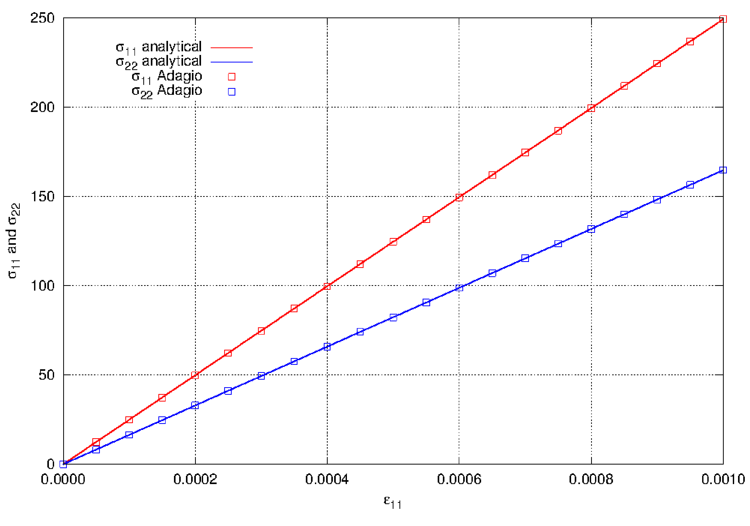
../../_images/elastic_uniaxial_stress.1.png — Fig. 4.1 The axial stress component \(\sigma_{11}\) in uniaxial stress using the elastic model.

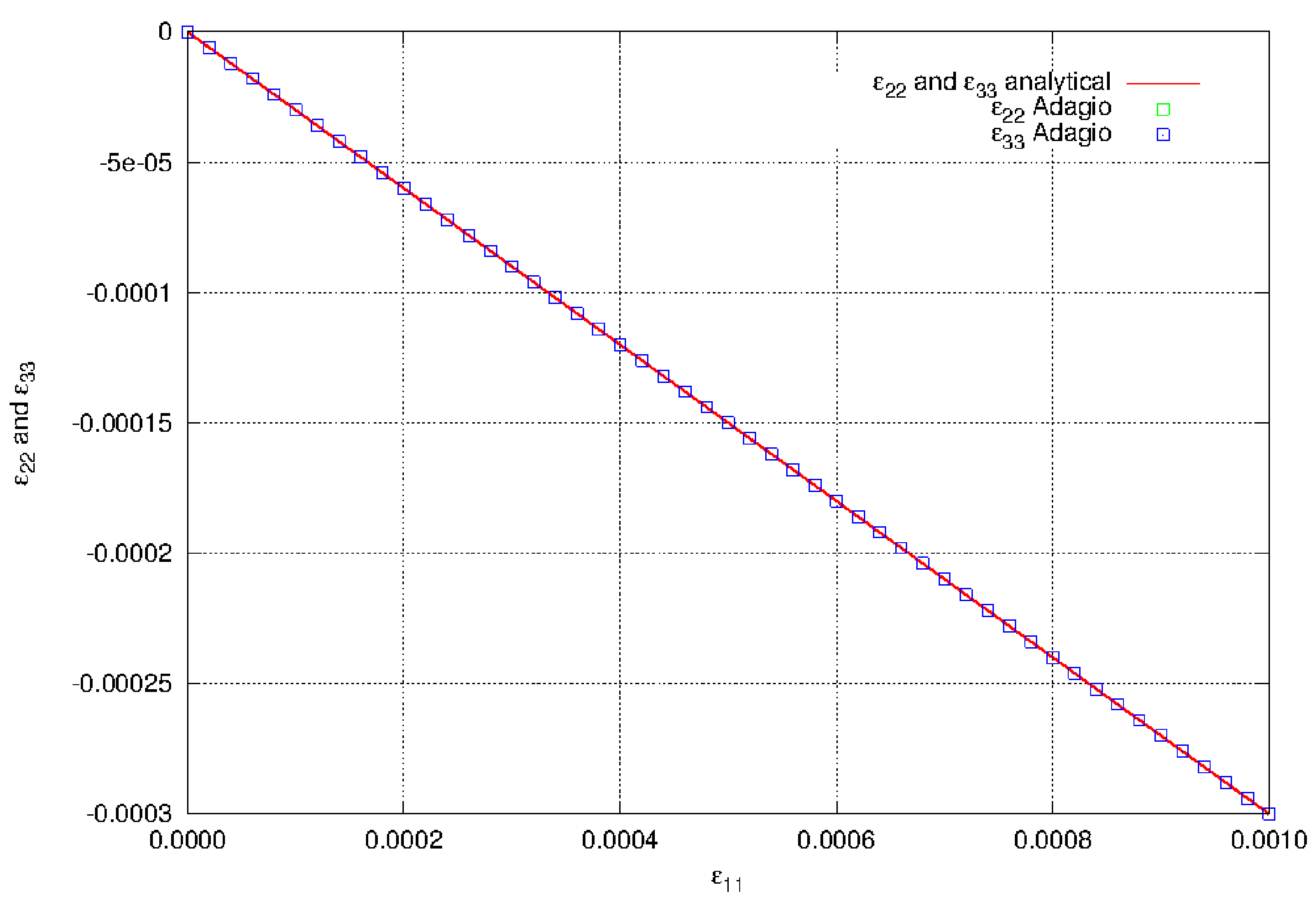
../../_images/elastic_uniaxial_stress.2.png — Fig. 4.2 The lateral strain components \(\varepsilon_{22}\) and \(\varepsilon_{33}\) in uniaxial stress using the elastic model.

4.3.3.2. Biaxial Stress

The elastic model is verified in biaxial stress. Biaxial stress is a plane stress state where \(\sigma_{11} = \sigma_{1}\), \(\sigma_{22} = \sigma_{2}\), and all other stress components are zero. The problem is displacement controlled in the \(x_{1}\) and \(x_{2}\) directions. If the applied strains are \(\varepsilon_{11} = \varepsilon\) and \(\varepsilon_{22} = \alpha\varepsilon\) where \(\alpha \in [0,1]\), then the applied displacements are

\[\begin{split}u_{1} & = \lambda_{1} - 1 \;\;\; ; \;\;\; \lambda_{1} = \exp(\varepsilon) \\ u_{2} & = \lambda_{2} - 1 \;\;\; ; \;\;\; \lambda_{2} = \exp(\alpha\varepsilon).\end{split}\]

In the following results, \(\alpha\) will be taken to be 0.45. For the plane stress state, we have \(\sigma_{33} = 0\), which allows us to solve for \(\varepsilon_{33}\)

\[\varepsilon_{33} = -\frac{\nu}{1-\nu}\left( 1+\alpha \right) \varepsilon.\]

The component \(\varepsilon_{33}\) is shown in Fig. 4.3. The in-plane stress components are

\[\begin{split}\sigma_{11} & = \frac{E}{1-\nu^{2}} \left( 1 + \alpha\nu \right)\varepsilon \\ \sigma_{22} & = \frac{E}{1-\nu^{2}} \left( \alpha + \nu \right)\varepsilon.\end{split}\]

The in-plane stress components are shown in Fig. 4.4.

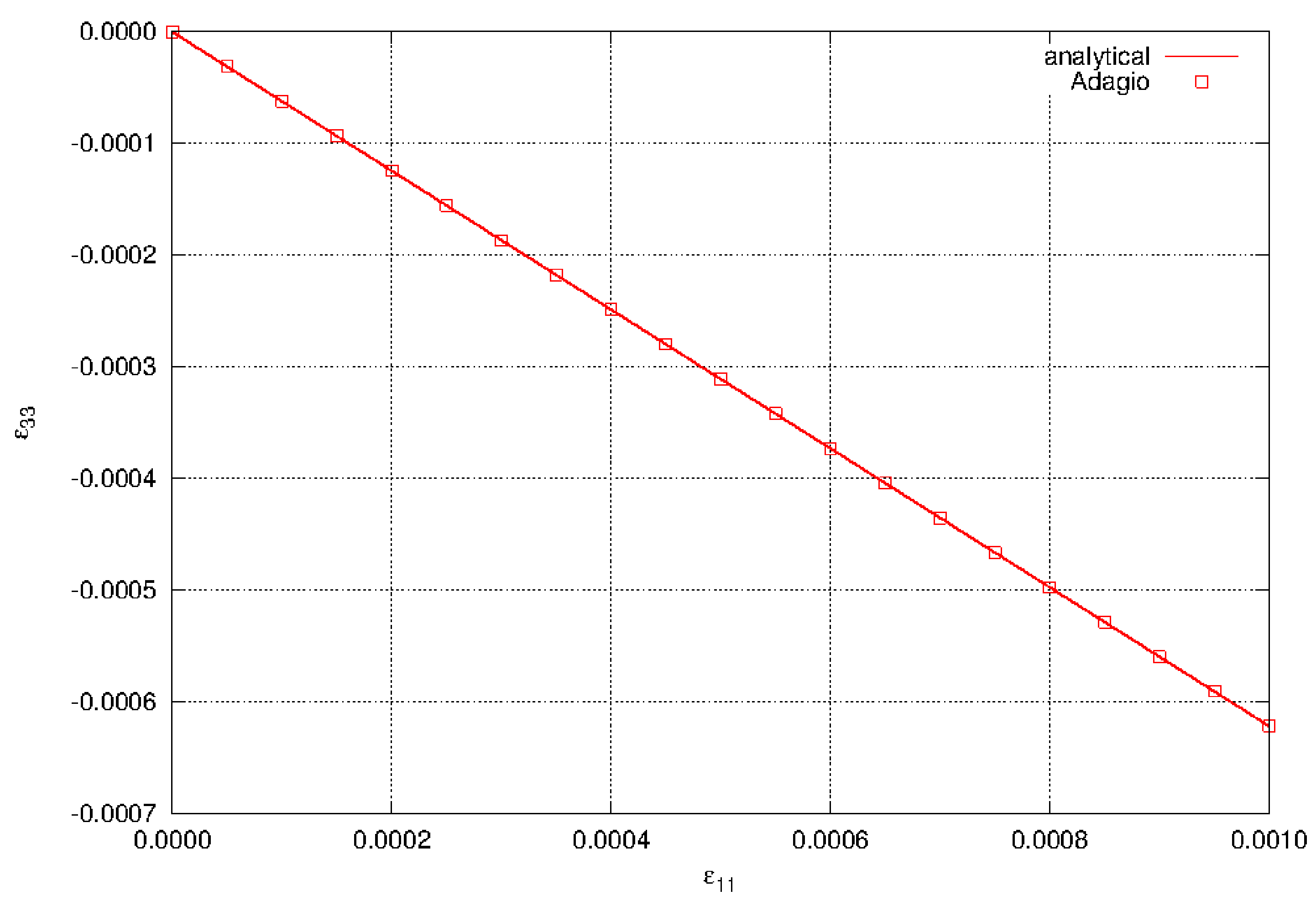
../../_images/elastic_biaxial_stress.2.png — Fig. 4.3 The strain component \(\varepsilon_{33}\) in biaxial stress using the elastic model.

../../_images/elastic_biaxial_stress.1.png — Fig. 4.4 The normal stress components \(\sigma_{11}\) and \(\sigma_{22}\) in biaxial stress using the elastic model.

4.3.3.3. Pure Shear

The elastic model is verified in pure shear. Pure shear gives a stress state where \(\sigma_{12}\) is the only non-zero stress component. The problem is completely displacement controlled and the applied shear strain is \(\varepsilon_{12} = \varepsilon (t)\).

The shear stress in the problem is

\[\sigma_{12} = 2\mu \varepsilon\]

The shear stress-strain response is shown in Fig. 4.5.

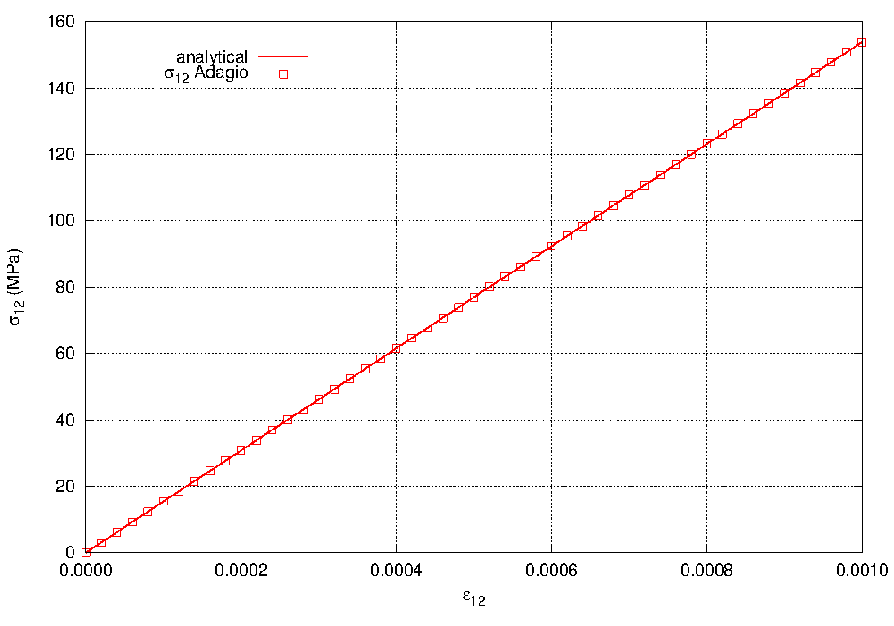
../../_images/elastic_pure_shear.png — Fig. 4.5 The shear stress component \(\sigma_{12}\) in pure shear using the elastic model.

4.3.3.4. Performance

The performance of the elastic model was analyzed using the material point driver. The elastic model was run in uniaxial strain for 1 billion calculations and the CPU time was recorded using clock() method in the time.h header. The start and end times are found and the CPU time is calculated by dividing the difference by the variable CLOCKS_PER_SECOND.

Since the CPU times will depend on many things outside of the actual code, a set of times were generated as a baseline. For this task the 1 billion calculations were performed 100 times. With the 100 CPU times the mean and standard deviation were calculated. Next we assume a normal distribution of CPU times and the normal distribution is generated.

Subsequent performance tests involve generating 10 sets of the 1 billion calculations. This much smaller data set is used to generate its own mean and standard deviation. If this mean is within 3 standard deviations of the baseline mean, then the performance of the model is assumed to be identical to that of the baseline model.

4.3.4. User Guide

BEGIN PARAMETERS FOR MODEL ELASTIC
  #
  # Elastic constants
  #
  YOUNGS MODULUS = <real>
  POISSONS RATIO = <real>
  SHEAR MODULUS  = <real>
  BULK MODULUS   = <real>
  LAMBDA         = <real>
  TWO MU         = <real>
END [PARAMETERS FOR MODEL ELASTIC]

There are no output variables available for the elastic model. For information about the elastic model, consult [[4]].