4.16. Barlat Plasticity Model
4.16.1. Theory
The Barlat plasticity model is a hypoelastic, rate-independent plasticity model. The underlying yield surface is both anisotropic and non-quadratic [[1]]. With respect to the former, linear transformations of the deviatoric stress are used to capture texture and anisotropy effects. The rate form of this model assumes an additive split of the rate of deformation into an elastic and plastic part
The stress rate only depends on the elastic rate of deformation
where \(\mathbb{C}_{ijkl}\) are the components of the fourth-order, isotropic elasticity tensor.
To describe anisotropy in the yield-behavior, two linear transformation tensors, \(C^{\prime}_{ijkl}\) and \(C^{\prime\prime}_{ijkl}\), are introduced such that,
with \(s_{ij}\) being the deviatoric stress tensor (\(s_{ij}=\sigma_{ij}-1/3\sigma_{kk}\delta_{ij}\)) and \(s_{ij}^{\prime}\) and \(s_{ij}^{\prime\prime}\) being transformed stresses. Two transformations are used to capture both the anisotropy of the yield surface and flow rule. In Voigt notation the two transformation tensors are given as,
Alternatively, the transformed stresses may be written in terms of the Cauchy stress tensor as,
where \(L^{\prime}_{ijkl}=C^{\prime}_{ijmn}I_{mnkl}\) and \(L^{\prime\prime}_{ijkl}=C^{\prime\prime}_{ijmn}I_{mnkl}\). In this case, \(I_{ijkl}\) is the symmetric deviatoric projection tensor and takes the form of,
In reduced form,
and an analogous expression may be written for \(L^{\prime\prime}_{ijkl}\).
The yield surface, \(f\), is given as,
in which \(\phi\left(\sigma_{ij}\right)\) is the effective stress and \(\bar{\sigma}\left(\bar{\varepsilon}^p\right)\) is the current yield stress that may depend on rate and/or temperature. The effective stress is written in terms of the principal transformed stresses (\(s^{\prime}_i\) and \(s^{\prime\prime}_i\), respectively) and the yield surface exponent, \(a\), as,
An example of such a yield surface is given in Fig. 4.75 along with examples of previously presented (von Mises, Hosford, Hill) surfaces. The presented Barlat surface corresponds to that of 2090-T3 aluminum first characterized by Barlat et al. [[1]]. In Fig. 4.75, both the anisotropy and non-quadratic nature of the yield surface is evident leading to differing strengths and flow directions at various stresses from any of the other models.
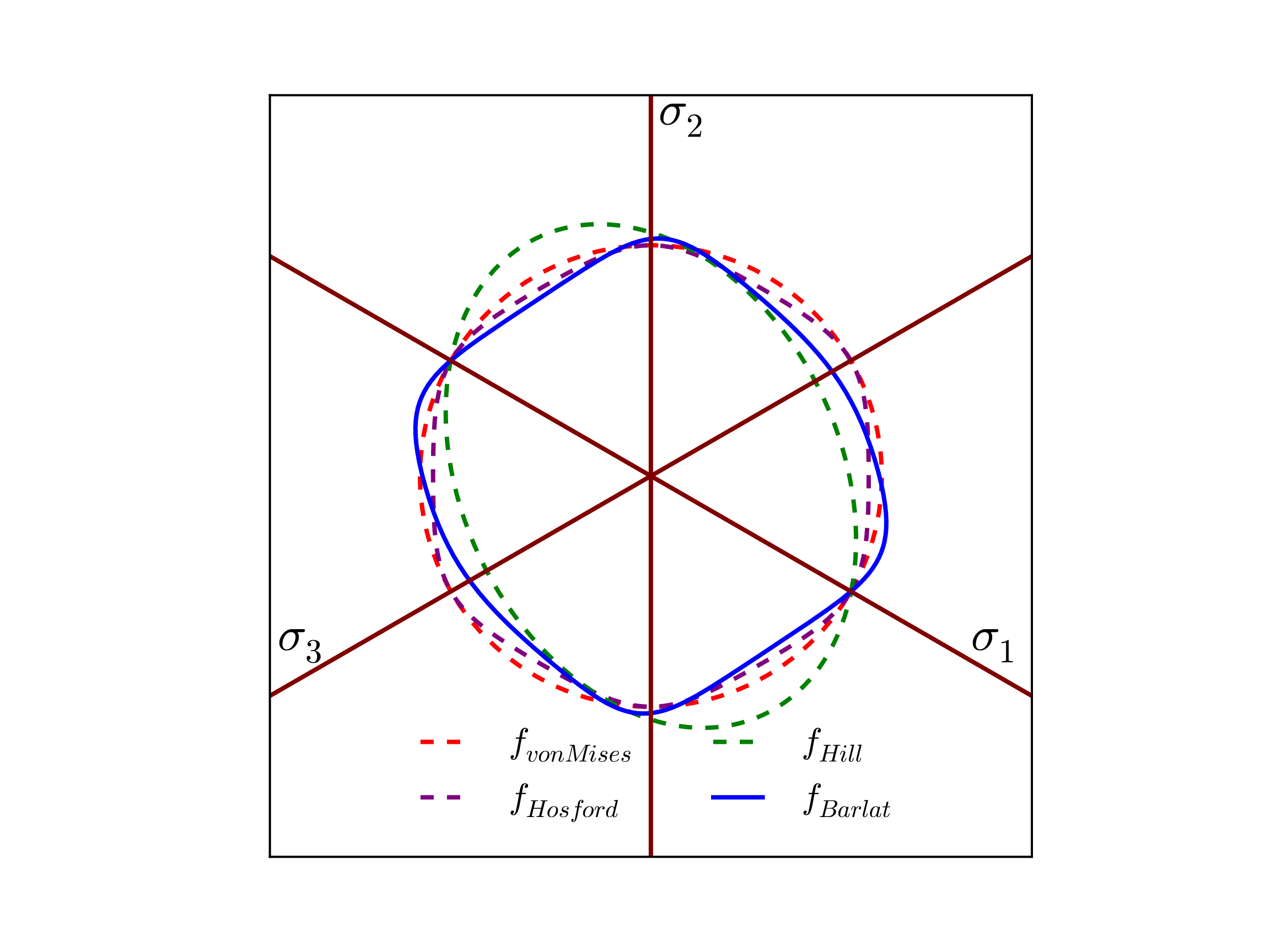
Fig. 4.75 Example Barlat yield surface, \(f_{Barlat}\left(\sigma_{ij},\bar{\varepsilon}^p=0\right)\), of 2090-T3 aluminum presented in the deviatoric \(\pi\)-plane. Comparison von Mises (\(J_2\)), Hosford (with \(a=8\)), and Hill surfaces are also presented for comparison.
The orientation of the principal material axes with respect to the global Cartesian axes may be specified by the user. First, a rectangular or cylindrical reference coordinate system is defined. Spherical coordinate systems are not currently implemented for the Barlat model. The material coordinate system can then be defined through two successive rotations about axes in the reference rectangular or cylindrical coordinate system. In the case of the cylindrical coordinate system this allows the principal material axes to vary point-wise in a given element block.
The plastic rate of deformation, as with the isotropic models, assumes associated flow
in which \(\dot{\gamma}\) is the consistency multiplier. Given the form for \(\phi\), \(\dot\gamma\) is equal to the rate of the equivalent plastic strain, \(\dot{\bar{\varepsilon}}^{p}\). As the yield surface is cast in transformed stress space, determining the flow direction in Cartesian space may be done via the chain rule (details may be found in [[2]]) leading to an expression of the form,
For more information about the Barlat plasticity model, consult [[1], [2]]. Additional discussion on options for failure models and adiabatic heating may be found in [[3], [4]] and [[5]], respectively.
4.16.1.1. Plastic Hardening
Plastic hardening refers to increases in the flow stress, \(\bar{\sigma}\), with plastic deformation. As such, hardening is described via a functional relationship between the flow stress and isotropic hardening variable (effective plastic strain), \(\bar{\sigma}\left(\bar{\varepsilon}^p\right)\). Over the course of nearly a century of work in metal plasticity, a variety of relationships have been proposed to describe the interactions associated with different physical interpretations, deformation mechanisms, and materials. To enable the utilization of the same plasticity models for different material systems, a modular implementation of plastic hardening has been adopted such that the analyst may select different hardening models from the input deck thereby avoiding any code changes or user subroutines. In this section, additional details are given for the different models to enable the user to select the appropriate choice of model. Note, the models being discussed here are only for isotropic hardening in which the yield surface expands. Kinematic hardening in which the yield surface translates in stress-space with deformation and distortional hardening where the shape of the yield surface changes shape with deformation are not treated. For a larger discussion of the phenomenology and history of different hardening types, the reader is referred to [[6], [7], [8]].
Given the ubiquitous nature of these hardening laws in computational plasticity, some (if not most) of this material may be found elsewhere in this manual. Nonetheless, the discussion is repeated here for the convenience of the reader.
4.16.1.1.1. Linear
Linear hardening is conceptually the simplest model available in LAMÉ. As the name implies, a linear relationship is assumed between the hardening variable, \(\bar{\varepsilon}^p\), and flow stress. The hardening modulus, \(H^{\prime}\), is a constant giving the rate of change of flow stress with plastic flow. The flow stress expression may therefore be written,
The simplicity of the model is its main feature as the constant slope,
makes the model attractive for analytical models and cheap for computational implementations (e.g. radial return algorithms require only a single correction step). Unfortunately, the simplicity of the representation also means that it has limited predictive capabilities and can lead to overly stiff responses.
4.16.1.1.2. Power Law
Another common expression for isotropic hardening is the power-law hardening model. Due to its prevalence, a dedicated ELASTIC-PLASTIC POWER LAW HARDENING model may be found in LAMÉ (see Section 4.8.1). This expression is given as,
in which \(<\cdot>\) are Macaulay brackets, \(\varepsilon_L\) is the Luders strain, \(A\) is a fitting constant, and \(n\) is an exponent typically taken such that \(0<n\leq1\). The Luders strain is a positive, constant strain value (defaulted to zero) giving an initially perfectly plastic response in the plastic deformation domain (see Fig. 4.20). The derivative is then simply,
Note, one difficulty in such an implementation is that when the effective equivalent plastic strain is zero, numerical difficulties may arise in evaluating the derivative and necessitate special treatment of the case.
4.16.1.1.3. Voce
The Voce hardening model (sometimes referred to as a saturation model) uses a decaying exponential function of the equivalent plastic strain such that the hardening eventually saturates to a specified value (thus the name). Such a relationship has been observed in some structural metals giving rise to the popularity of the model. The hardening response is given as,
in which \(A\) is a fitting constant and \(n\) is a fitting exponent controlling how quickly the hardening saturates. Importantly, the derivative is written as,
and is well defined everywhere giving the selected form an advantage over the aforementioned power law model.
4.16.1.1.4. Johnson-Cook
The Johnson-Cook hardening model is a variant of the classical Johnson-Cook [[9], [10]] expression. In this instance, the temperature-dependence is neglected to focus on the rate-dependent capabilities while allowing for arbitrary isotropic hardening forms via the use of a user-defined hardening function. With these assumptions, the flow stress may be written as,
in which \(\tilde{\sigma}_y\left(\bar{\varepsilon}^p\right)\) is the user-specified rate-independent hardening function, \(C\) is a fitting constant and \(\dot{\varepsilon}_0\) is a reference strain rate. The Macaulay brackets ensure the material behaves in a rate independent fashion when \(\dot{\bar{\varepsilon}}^p < \dot{\varepsilon}_0\).
4.16.1.1.5. Power Law Breakdown
Like the Johnson-Cook formulation, the power-law breakdown model is also rate-dependent. Again, a multiplicative decomposition is assumed between isotropic hardening and the corresponding rate-dependence dependent. In this case, however, the functional form is derived from the analysis of Frost and Ashby [[11]] in which power-law relationships like those of the Johnson-Cook model cease to appropriately capture the physical response. The form used here is similar to the expression used by Brown and Bammann [[12]] and is written as,
with \(\tilde{\sigma}_y\left(\bar{\varepsilon}^p\right)\) being the user supplied rate independent expression, \(g\) is a model parameter related to the activation energy required to transition from climb to glide-controlled deformation, and \(m\) dictates the strength of the dependence.
4.16.2. Implementation
Like the Hill and Hosford models, the Barlat plasticity model uses a elastic predictor-inelastic corrector closest point projection (CPP) return mapping algorithm (RMA) for integration. Details of the numerical scheme and forms of the necessary derivatives may be found in the work of Scherzinger [[2]]. For this approach, given a rate of deformation, \(d_{ij}\), and a time step, \(\Delta t\), a trial stress state is calculated based on an elastic response
If the trial stress state lies outside the yield surface, i.e. if \(\phi(T_{ij}^{tr}) > \bar{\sigma}\), then the model uses an implicit, backward Euler algorithm to return the stress to the yield surface. To perform this task, two nonlinear equations need to be solved. The first is associated with the satisfaction of the flow-rule and ensures that the plastic strain increment is in the correct direction. Such a relation leads to a residual of the form,
while the second equation to be addressed enforces that the converged stress state is on the yield surface and is written as,
The primary method for solving these equations is a Newton-Raphson algorithm. With \(\Delta \gamma\) (which is equal to \(\Delta\bar{\varepsilon}^{p}\)) and \(T_{ij}\) being the solution variables, an iterative algorithm is utilized such that
with \(\Delta\gamma^{(0)} = 0\) and \(T_{ij}^{(0)} = T_{ij}^{tr}\). The plastic rate of deformation correction is then simply
After linearizing the residual and consistency equations (Equations (4.54) and (4.55)), the set of nonlinear equations may be solved for the correction increments leading to expressions of the form,
and \(\mathcal{L}^{\left(k\right)}_{ijkl}\) is the Hessian of the RMA problem (not the yield surface) and is given as,
and \(\mathbb{S}_{ijkl}=\mathbb{C}_{ijkl}^{-1}\).
Unfortunately, a straightforward Newton-Raphson algorithm does not always converge, so the RMA is augmented with a line search algorithm producing modified incrementation relations with
where \(\alpha \in (0,1]\) is the line search parameter which is determined from certain convergence considerations. If \(\alpha = 1\) then the Newton-Raphson algorithm is recovered. The line search algorithm greatly increases the reliability of the return mapping algorithm.
4.16.3. Verification
To verify the Barlat plasticity model a similar approach to that used for the Hill plasticity model (Section 4.15.3) is utilized.
Additional verification exercises for the various failure models and adiabatic heating capabilities may be found in [[3], [4]] and [[5]], respectively.
Specifically, both uniaxial stress and pure shear loadings are considered. To this end, the response of a 2090-T3 aluminum [[1]] with Voce hardening of the form,
is used. The corresponding elastic, plastic, and anisotropy model parameters are given in Table 4.22.
\(E\) |
70 GPa |
\(\nu\) |
0.25 |
\(a\) |
8 |
\(\sigma_{y}\) |
200 MPa |
\(A\) |
200 MPa |
\(b\) |
20 |
\(c^{\prime}_{12}\) |
-0.069888 |
\(c^{\prime\prime}_{12}\) |
0.981171 |
\(c^{\prime}_{13}\) |
0.936408 |
\(c^{\prime\prime}_{13}\) |
0.476741 |
\(c^{\prime}_{21}\) |
0.079143 |
\(c^{\prime\prime}_{21}\) |
0.575316 |
\(c^{\prime}_{23}\) |
1.003060 |
\(c^{\prime\prime}_{23}\) |
0.866827 |
\(c^{\prime}_{31}\) |
0.524741 |
\(c^{\prime\prime}_{31}\) |
1.145010 |
\(c^{\prime}_{32}\) |
1.363180 |
\(c^{\prime\prime}_{32}\) |
-0.079294 |
\(c^{\prime}_{44}\) |
1.023770 |
\(c^{\prime\prime}_{44}\) |
1.051660 |
\(c^{\prime}_{55}\) |
1.069060 |
\(c^{\prime\prime}_{55}\) |
1.147100 |
\(c^{\prime}_{66}\) |
0.954322 |
\(c^{\prime\prime}_{66}\) |
1.404620 |
Finally, the coordinate system used in these calculations is a rectangular coordinate system with the \(e^{1}_i,e^{2}_i,e^{3}_i\) axes aligned with the \(x,y,z\) axes.
4.16.3.1. Uniaxial Stress
First, the response of the material subject to a uniaxial stress is considered. As such, the Cauchy stress tensor takes the form \(\sigma_{ij}=\sigma\delta_{i1}\delta_{j1}\). In the transformed stress space, this uniaxial tensor becomes,
It is noted from (4.56) the that two transformed stress tensors are purely diagonal and therefore in a principal state. The actual ordering of the components into the corresponding principal stresses depends on the anisotropy coefficients. By inspection of Table 4.22 it is clear in this instance that tensors are already ordered (\(s^{\prime}_1=s^{\prime}_{11},~s^{\prime\prime}_1=s^{\prime\prime}_{11}\) etc.). With this observation, the effective stress may be reduced to,
where \(\omega\) is a constant dependent on model parameters and is written as,
4.16.3.1.1. Axial Stresses
To determine the axial stress, it is first noted that during plastic deformation,
where the fact that a tensile loading will be investigated (\(\sigma>0\)) is leveraged. The stress is then simply,
This shows that during plastic deformation the stress state can be calculated from the hardening law and anisotropy parameters.
To evaluate the axial stress, a relationship between the equivalent plastic strain and axial strain is needed. By noting the uniaxial stress state and equating the rate of plastic work, it is evident that,
which, when integrated, gives an implicit equation for the equivalent plastic strain that is written as
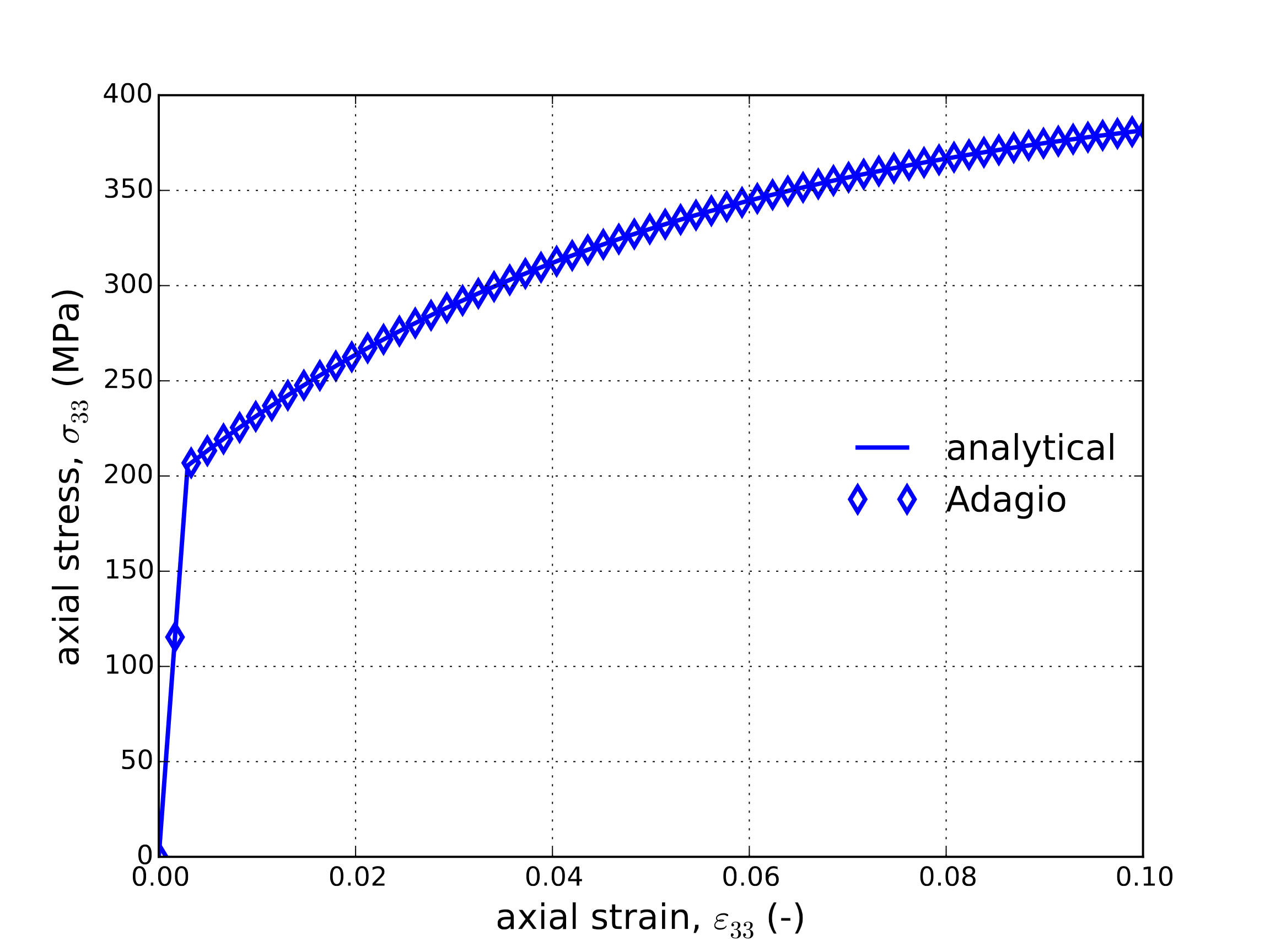
The equivalent plastic strain can then be used in (4.57) to find the axial stress, \(\sigma\). Corresponding stress-strain results determined analytically in this fashion and numerically via Adagio are presented below in Fig. 4.76.
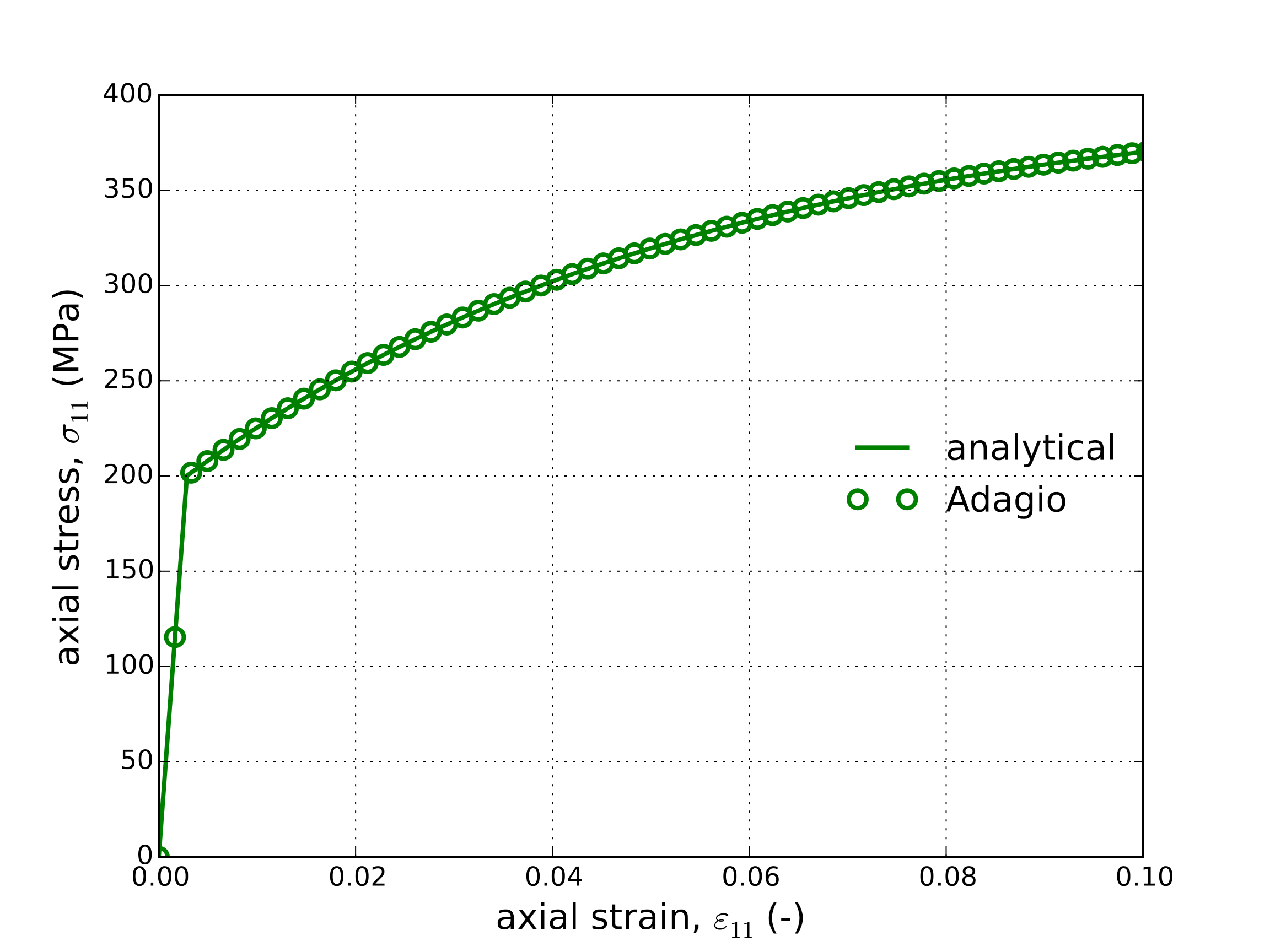
Fig. 4.76 Axial stress-strain response determined analytically and numerically for 2090-T3 aluminum using the Barlat plasticity model with Voce hardening.
4.16.3.1.2. Lateral Strains
To determine the plastic strain, the derivatives of the yield surface with respect to the Cauchy stress (\(\partial\phi/\partial\sigma_{ij}\)) are needed. From (4.53) it can be seen that these relations are quite complex and the reader is referred to [[2]] for a detailed discussion of how to rigorously evaluate these derivatives under arbitrary conditions. In this effort, the fact that the principal directions of the transformed stresses (\(\hat{e}^{k\prime}_i\) and \(\hat{e}^{k\prime\prime}_i\)) are aligned with the global coordinate system (\(\hat{e}^{1\prime}_i=e^1_i\) etc.) simplifies the problem sufficiently to allow for an analytical treatments. In this case,
With this observation, the lateral flow directions may be written as,
in which the various \(\partial\phi/\partial s^{\prime}_i\) derivatives are functions of the anisotropy coefficients and explicit forms may be found in [[2]].
The total strain is written simply as,
with the elastic strain being
and the plastic strains found via the flow rules as,
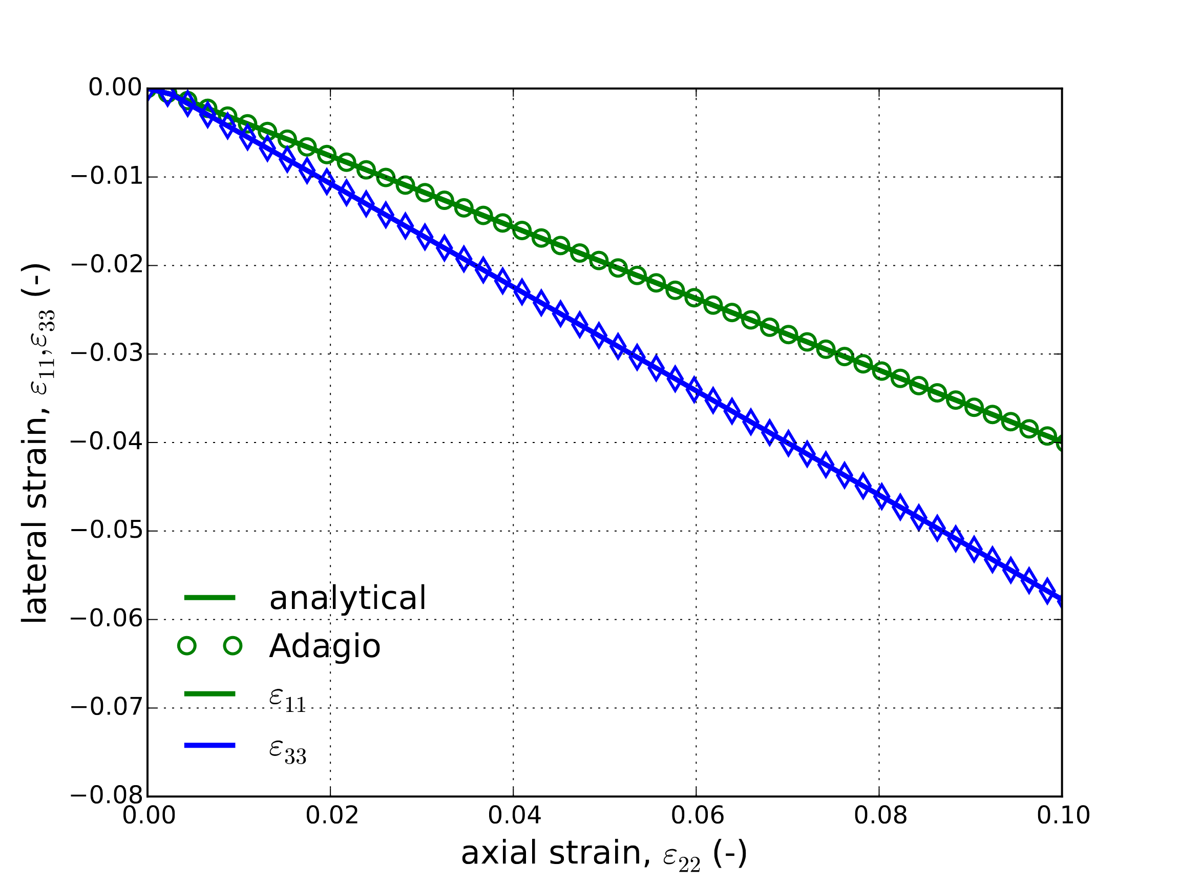
The flow directions were given previously in (4.59) and (4.60) while the equivalent plastic strain may be found via (4.58). Fig. 4.77 presents the lateral strains as a function of the axial. Clear agreement may be observed both in Fig. 4.76 and Fig. 4.77 verifying the model. Additionally, the effect of the anisotropy is plainly evident in Fig. 4.77 in which the two lateral strains differ by approximately a factor of four.
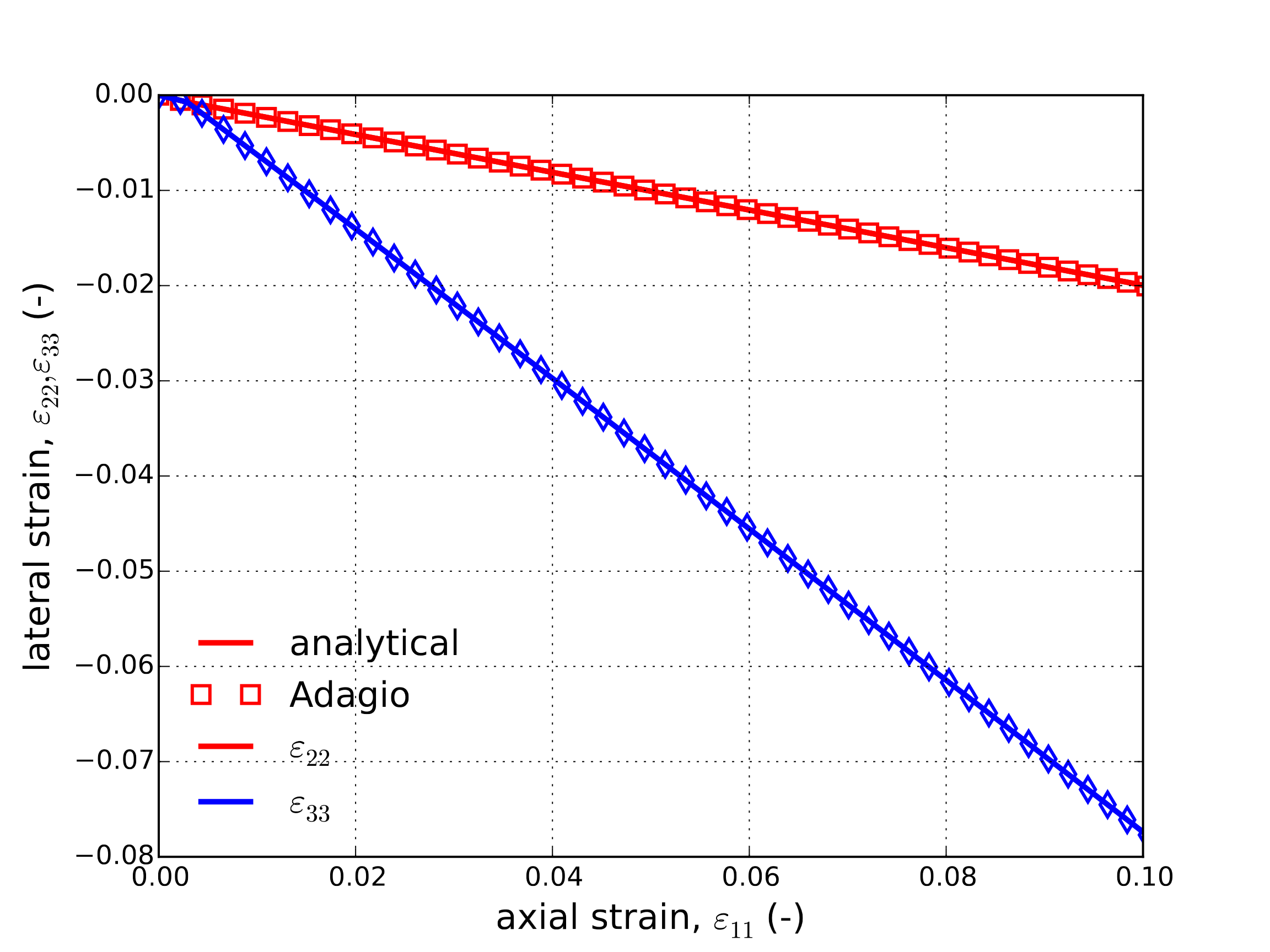
Fig. 4.77 Lateral strain as a function of axial strain of 2090-T3 aluminum with Voce hardening as determined by the Barlat plasticity model both analytically and numerically.
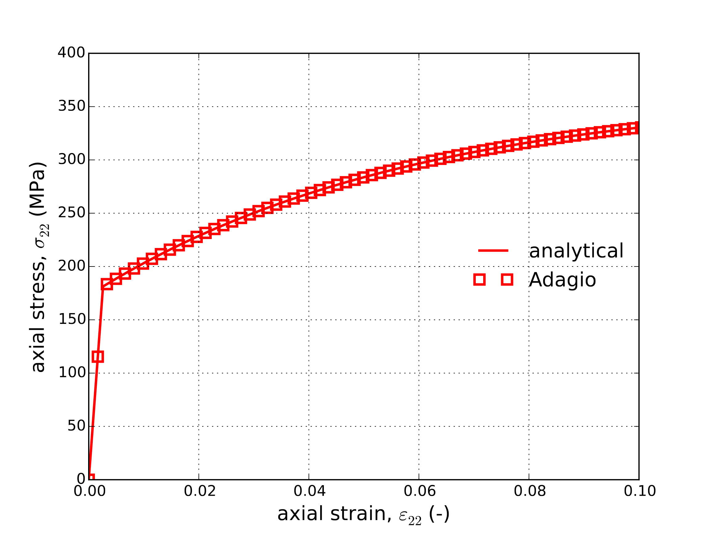
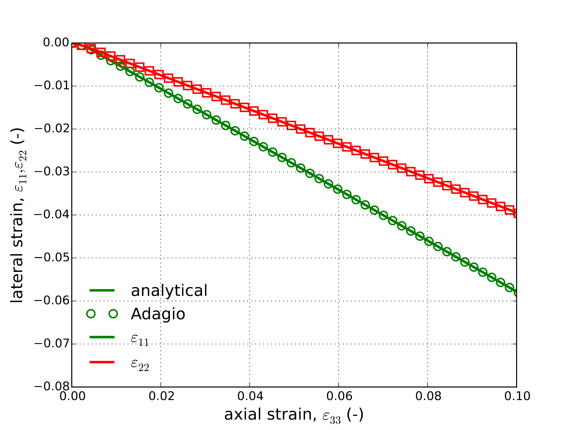
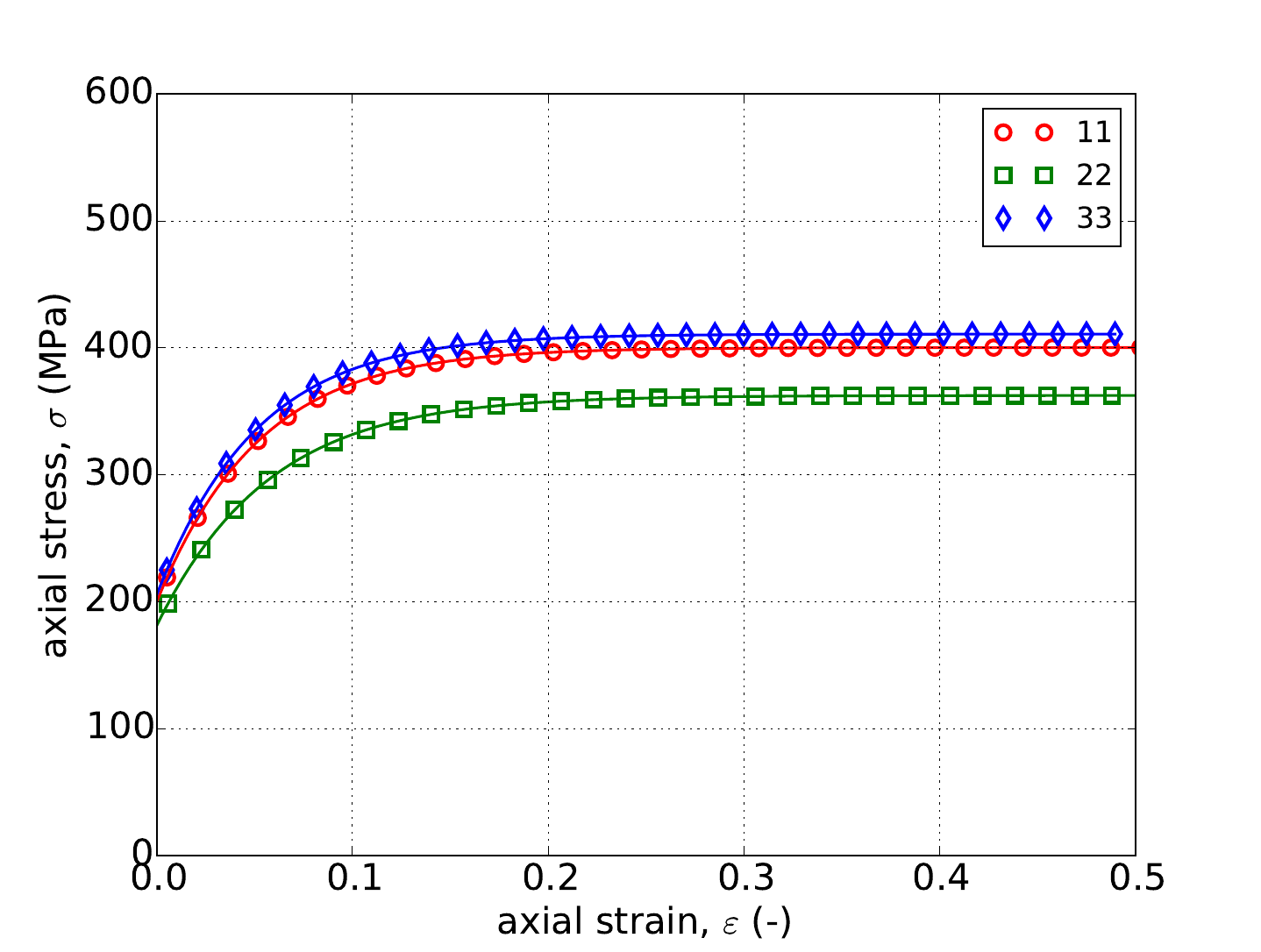
To test the other directions and further examine the anisotropic character of the model, the coordinate system rotation input options are used to align the 2 and 3 directions of the material with the applied load. Analytical expressions may be determined by similarly rotating the coefficients in the previous expressions, although these are not repeated here for brevity. The corresponding results for the loading aligned with the 2 and 3 directions are presented in Fig. 4.78 and Fig. 4.79, respectively. All of the results are given with respect to the original coordinate system to avoid confusion. Clear agreement between analytical and simulation results is noted in both cases further verifying the capabilities of the model. Importantly, by comparing the various stress-strain and lateral strain curves, the influence of the material and model anisotropy on the responses may readily be observed.
 Stress-strain
 Lateral strains
Fig. 4.78 Stress-strain (a) and lateral strain (b) responses of 2090-T3 aluminum with Voce hardening and the Barlat plasticity model. The material is rotated such that the loading is aligned with the 2 direction.
 Stress-strain
 Lateral strains
Fig. 4.79 Stress-strain (a) and lateral strain (b) responses of 2090-T3 aluminum with Voce hardening and the Barlat plasticity model. The material is rotated such that the loading is aligned with the 3 direction.
4.16.3.2. Pure Shear
In this section, the pure shear response of the Barlat model is interrogated to assess its performance under such conditions. Before proceeding, it is important to recall the ordering of the shear stresses in Sierra/SM. Specifically, the \(\sigma_{12},\ \sigma_{23},\) and \(\sigma_{31}\) stresses are associated with the 44, 55, and 66, respectively, anisotropy coefficients.
To explore the shear performance of the Barlat plasticity model, a stress tensor of the form \(\sigma_{ij}=\tau\left(\delta_{i1}\delta_{j2}+\delta_{i2}\delta_{j1}\right)\) is considered. The ordered principal stresses of the transformed stress tensors are,
thereby simplifying the effective stress to,
with
During plastic flow,
producing an expression for the stress in terms of equivalent plastic strain as,
A relationship between the equivalent plastic and axial strains may be determined by first considering the equivalency of plastic work,
Integrating leads to an implicit expression of the form,
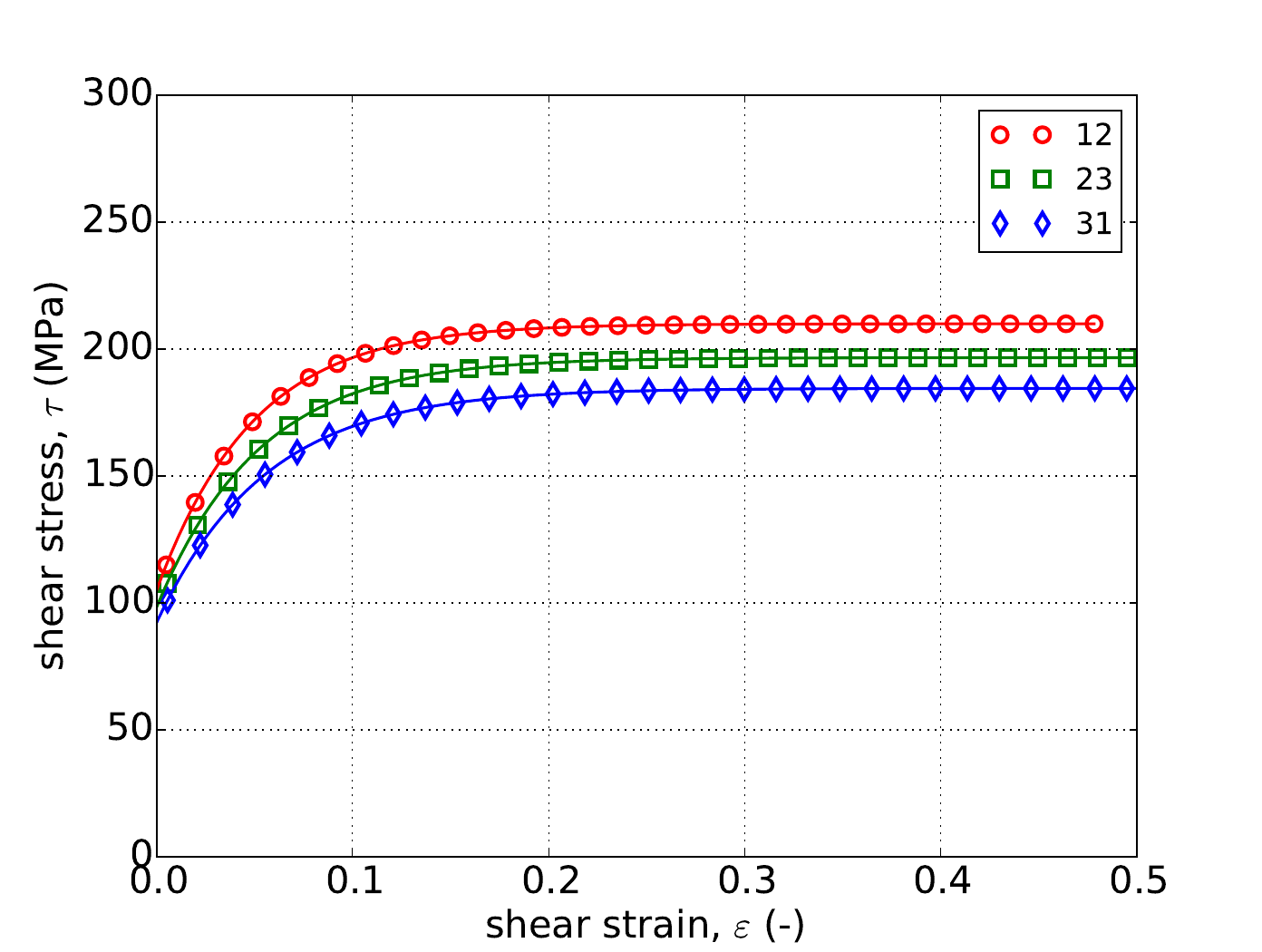
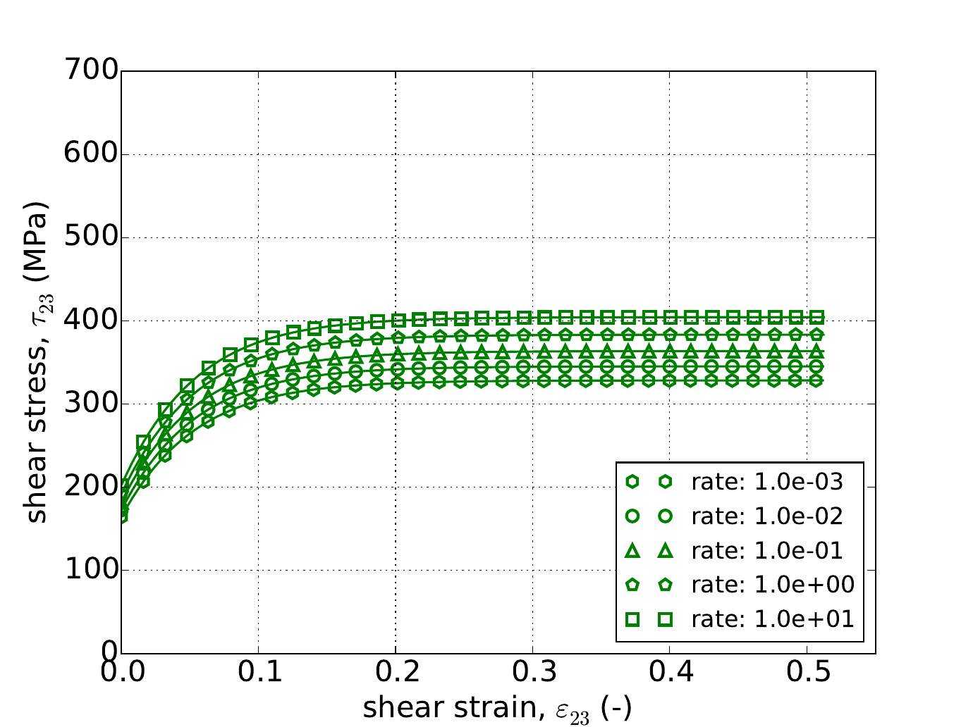
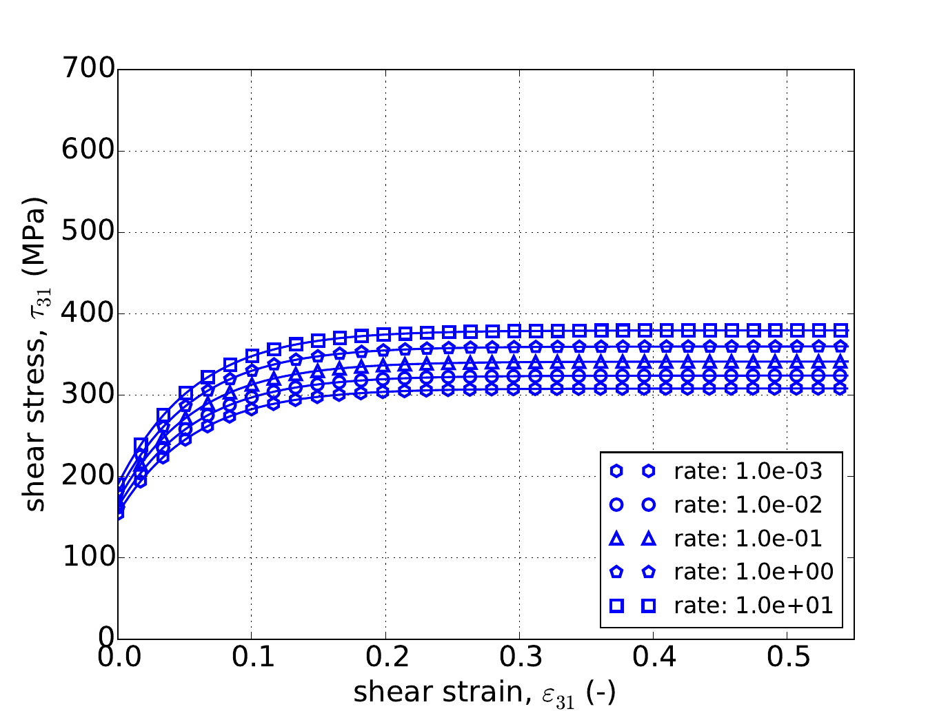
The preceding relations may be used to analytically determine the shear stress-strain response. Corresponding results, along with those produced by Adagio, are presented in Fig. 4.80. Shear responses are also presented for stress tensors of the form \(\sigma_{ij}=\tau\left(\delta_{2i}\delta_{3j}+\delta_{3i}\delta_{2j}\right)\) (23) and \(\sigma_{ij}=\tau\left(\delta_{1i}\delta_{3j}+\delta_{3i}\delta_{1j}\right)\) (31). Analytically, these results were determined by substituting the relevant anisotropy coefficients in (4.61)-(4.62). For the results from Adagio, the coordinate system input commands were used to rotate the material coordinate system accordingly.
In all the cases presented in Fig. 4.80 excellent agreement is noted. This not only verifies the performance of the current model under pure shear loadings but also demonstrates the impact of the anisotropy and exercises the coordinate system rotation capabilities.
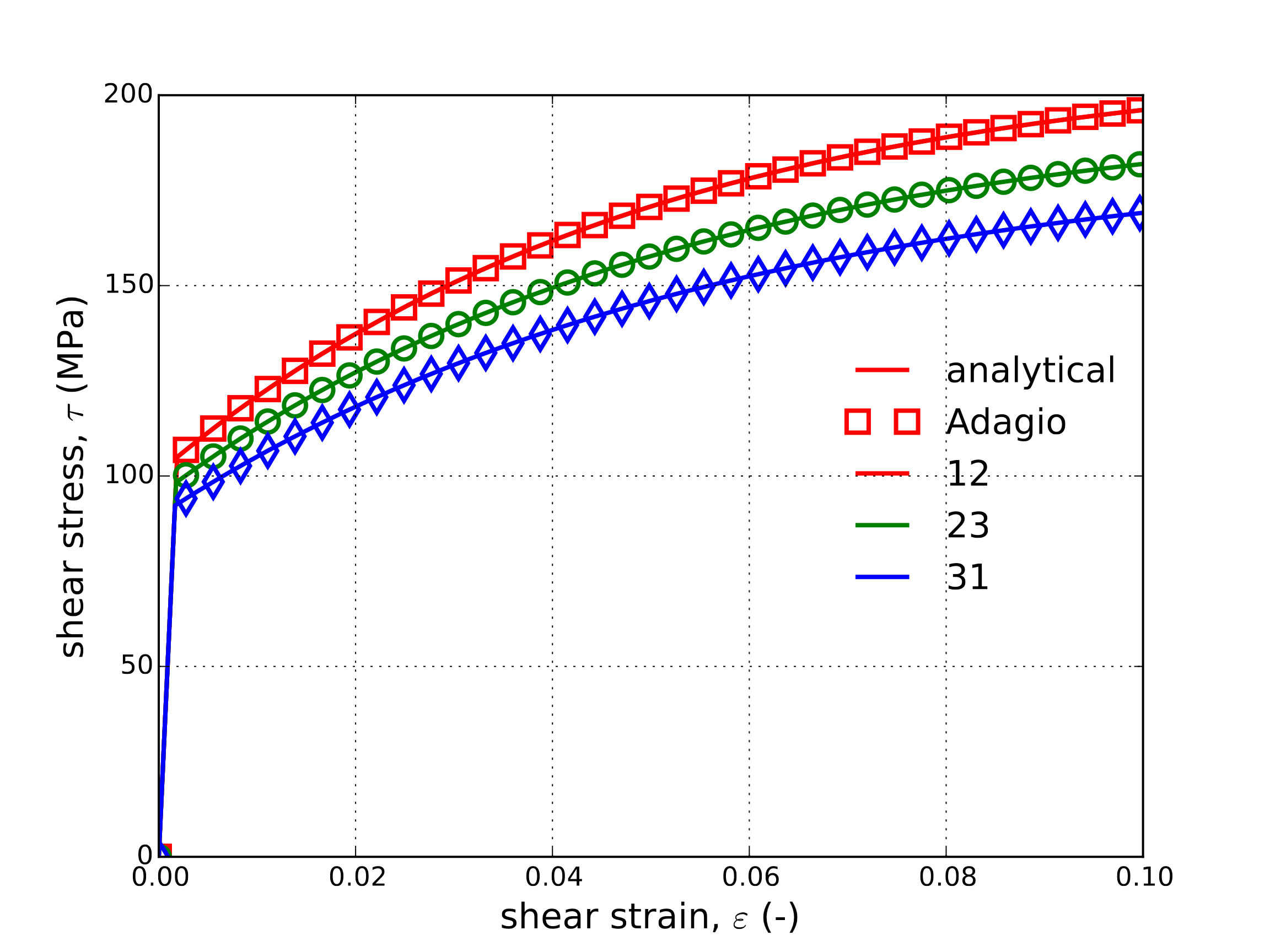
Fig. 4.80 Shear stress-strain results for 2090-T3 aluminum determined analytically and numerically by the Barlat plasticity model with Voce Hardening
4.16.3.3. Plastic Hardening
To verify the capabilities of the hardening models, rate independent and rate dependent alike, the constant equivalent plastic strain rate, \(\dot{\bar{\varepsilon}}^p\), uniaxial stress and pure shear verification tests described in Appendix A are utilized. In these simplified loading cases, the material state may be found explicitly as a function of time knowing the prescribed equivalent strain rate. For the rate independent cases, a strain rate of \(\dot{\bar{\varepsilon}}^p=1\times10^{-4} \text{s}^{-1}\) is used for ease in simulations although the selected rate does note affect the results. Through this testing protocol, the hardening models are not only tested at different rates but also in different principal material directions to consider the anisotropy of the Barlat yield surface. Additionally, the rate dependent models are tested for a wide range of strain rates (over five decades) with all three rate independent hardening functions (\(\tilde{\sigma}_y\) in the previous theory section). Although linear, Voce, and power-law rate independent representations are utilized in the rate dependent tests, in those cases the hardening models are prescribed via user-defined analytic functions. The rate independent verification exercises, on the other hand, examine the built-in hardening models. This distinction necessitates the different considerations and treatments.
The rate dependent and rate independent hardening coefficients are found in Table 4.23 while the remaining model parameters are unchanged from the previous verification exercises. For the current verification exercise, the rate independent hardening models (linear, Voce, and power-law) will first be considered and then the rate dependent forms (Johnson-Cook, power-law breakdown).
\(C\) |
0.1 |
\(\dot{\varepsilon}_0\) |
\(1\times 10^{-4}\) s\(^{-1}\) |
\(g\) |
0.21 s\(^{-1}\) |
\(m\) |
16.4 |
\(\tilde{H}_{\text{Linear}}\) |
200 MPa |
||
\(\tilde{A}_{\text{PL}}\) |
400 MPa |
\(\tilde{n}_{\text{PL}}\) |
0.25 |
\(\tilde{A}_{\text{Voce}}\) |
200 MPa |
\(\tilde{n}_{\text{Voce}}\) |
20 |
4.16.3.3.1. Linear
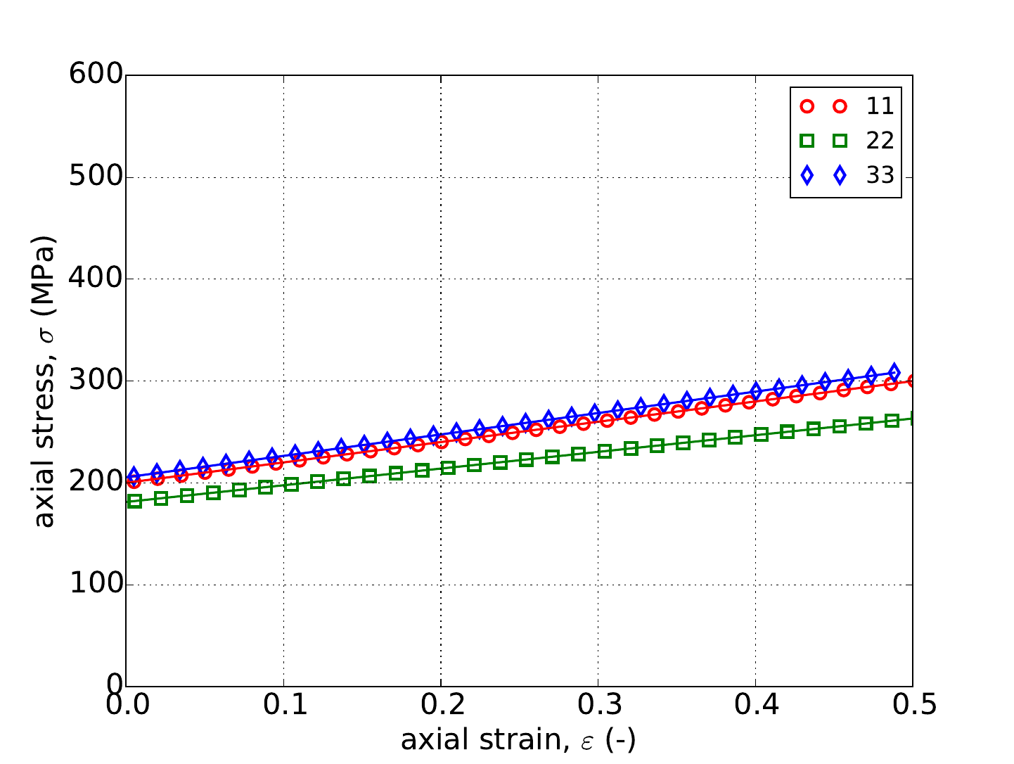
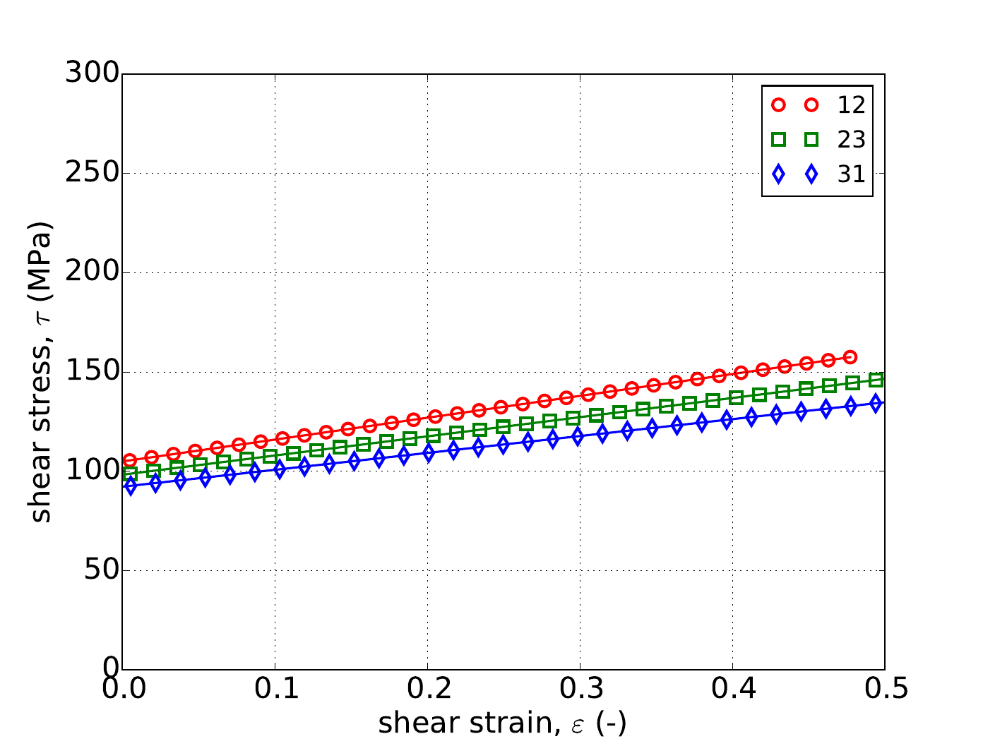
For the rate independent linear hardening model, verification is considered via the uniaxial stress and pure shear exercises of Appendix A. As the anisotropic Barlat yield surface is being used for this examination, the uniaxial stress response is determined for loading in three different principal material planes while the pure shear response is found along three shear planes. Results determined analytically and numerically are presented in Fig. 4.81. Clear agreement is evident between the dual solution approaches. Additionally, the linear response and constant tangent modulus during plastic deformation highlights the characteristic feature of the current model.
 Stress-strain
 Lateral strains
Fig. 4.81 Uniaxial stress-strain (a) and pure shear (b) responses of the Barlat plasticity model with rate independent, linear hardening. Solid lines are analytical while open symbols are numerical
4.16.3.3.2. Power-Law
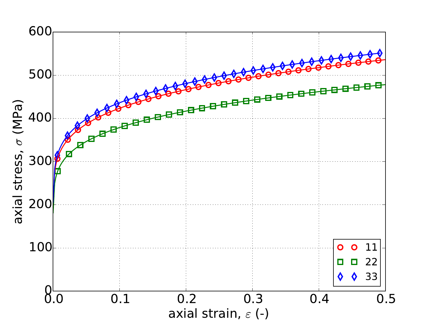
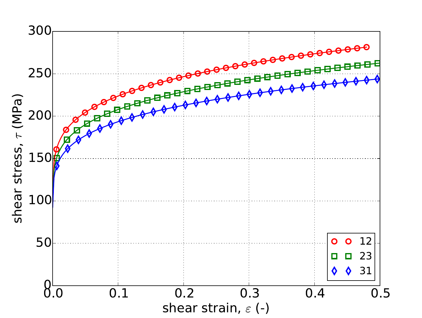
To probe the power-law rate independent hardening model, analytical and numerical results to the uniaxial stress and pure shear problems of Appendix A are determined. Given the anisotropic nature of the current model, responses are determined along the three principal and three shearing planes for the uniaxial stress and pure shear cases and all six cases are shown in Fig. 4.82. In considering Fig. 4.82, it is apparent that the numerical and analytical responses agree quite well verifying this specific response. These cases also highlight the initially stiff plastic response that eventually evolves into a more compliant linear like response that is associated with a power-law hardening model.
 Stress-strain
 Lateral strains
Fig. 4.82 Uniaxial stress-strain (a) and pure shear (b) responses of the Barlat plasticity model with rate independent, power-law hardening. Solid lines are analytical while open symbols are numerical.
4.16.3.3.3. Voce
Verifying the Voce model is addressed through the methods of Appendix A. To this end, analytical and numerical uniaxial stress and pure shear responses are determined along three different principal directions and shear planes, respectively. The results for these various cases are presented in Fig. 4.83 and unambiguous agreement is readily seen between the analytical and numerical results providing further credence to hardening model capabilities. Responses in Fig. 4.83 also exhibit the clear saturation of hardening with sufficient plastic strain that is usually associated with the Voce model.
 Stress-strain
 Lateral strains
Fig. 4.83 Uniaxial stress-strain (a) and pure shear (b) responses of the Barlat plasticity model with rate independent, Voce hardening. Solid lines are analytical while open symbols are numerical.
4.16.3.3.4. Johnson-Cook
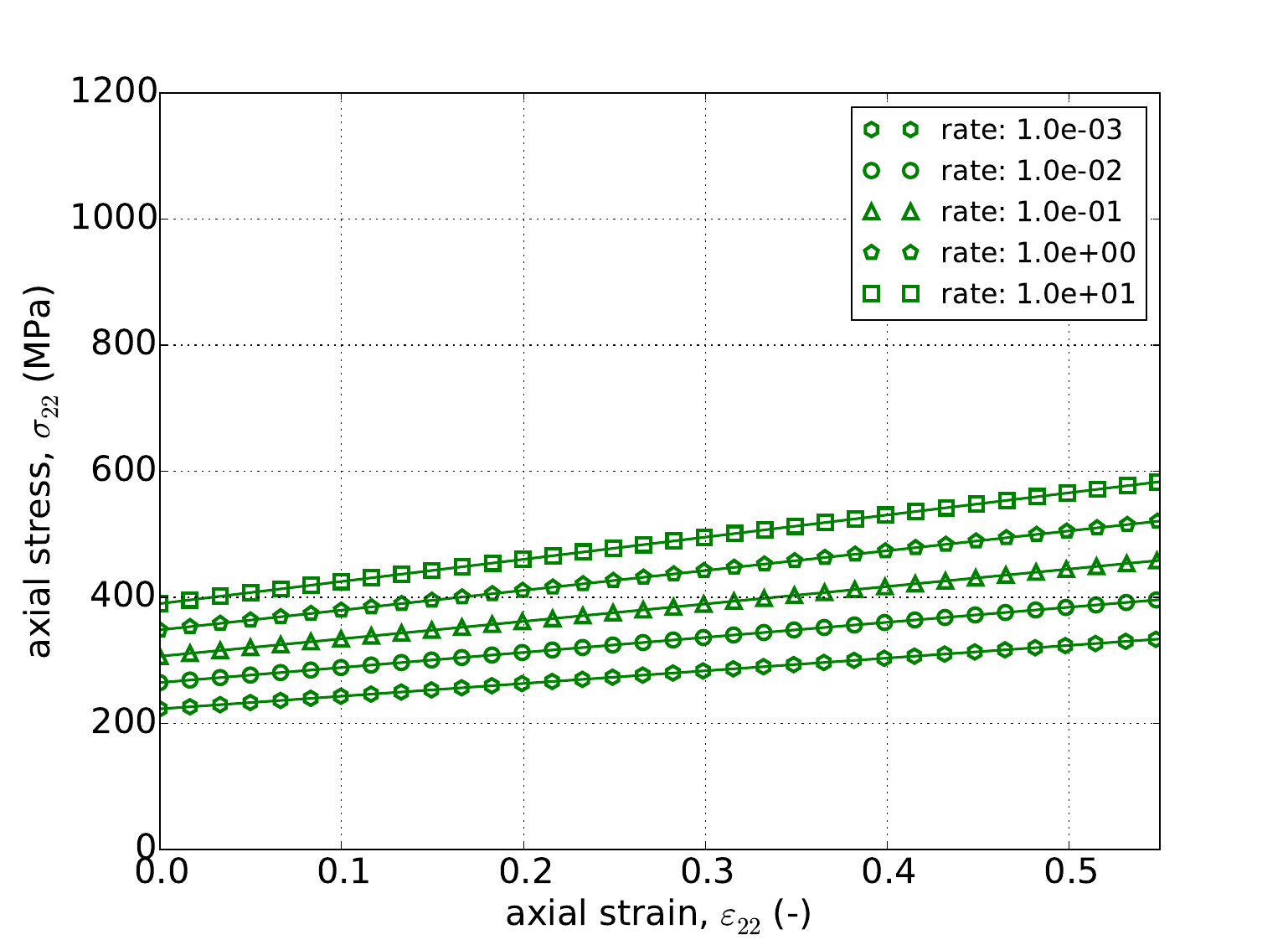
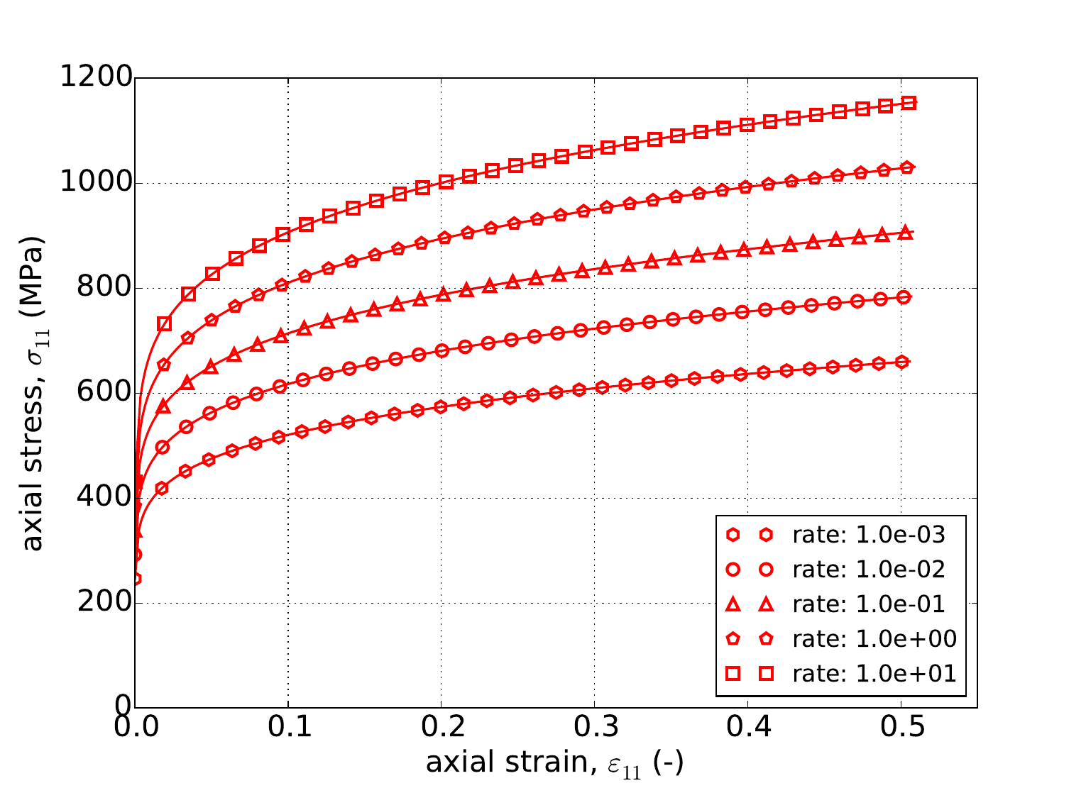
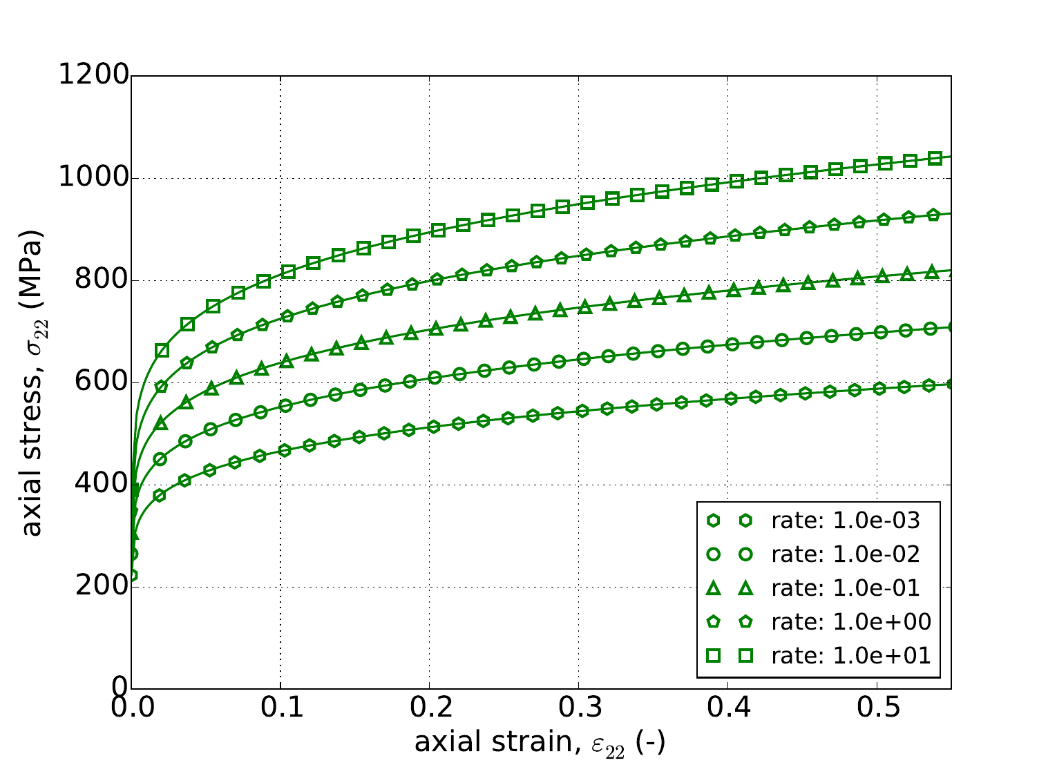
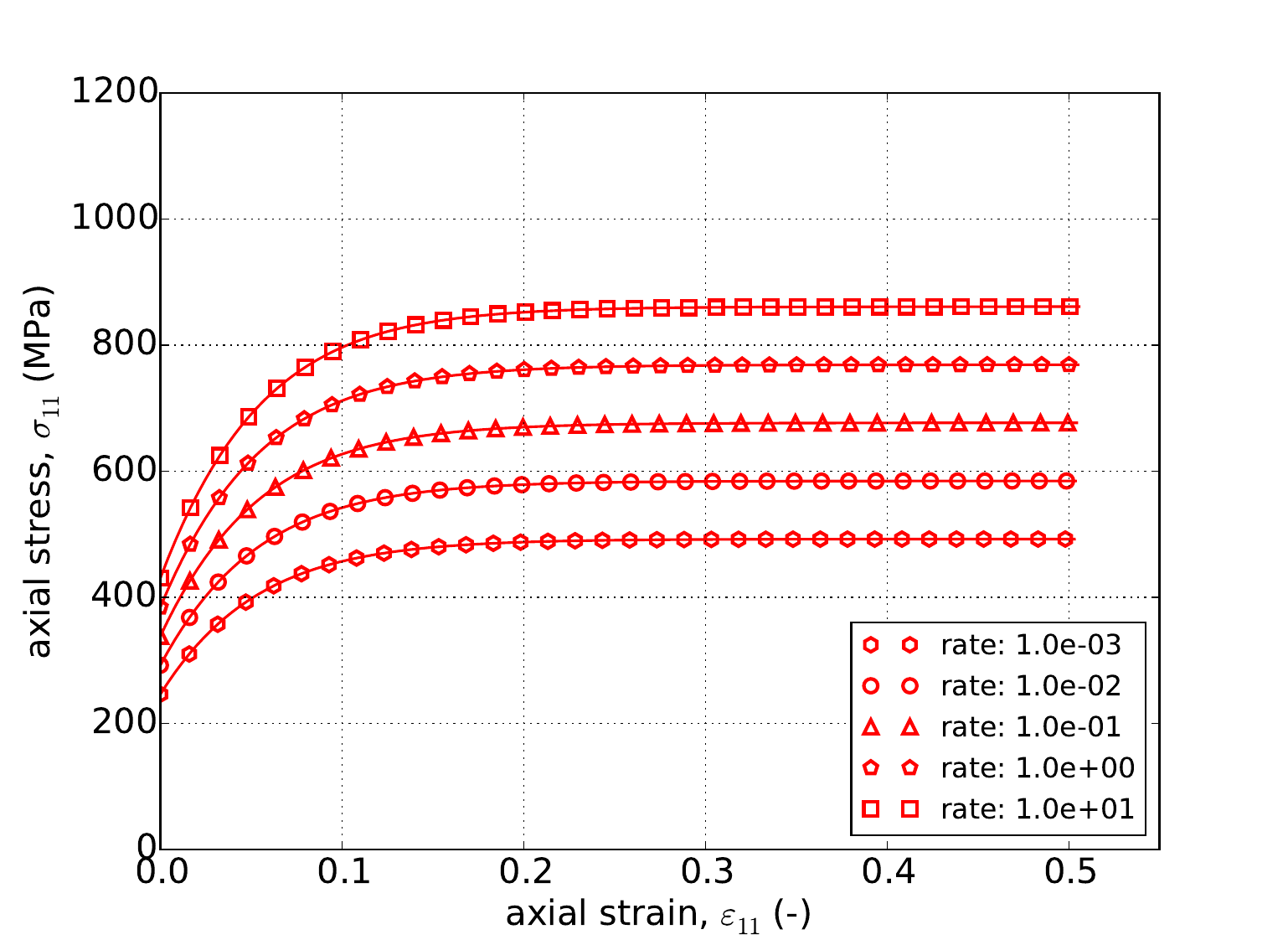
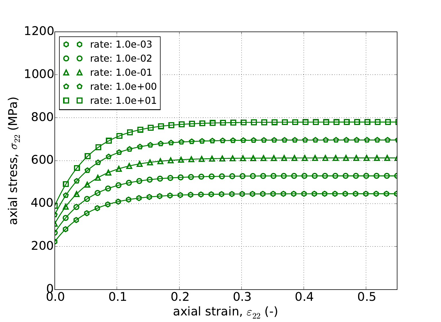
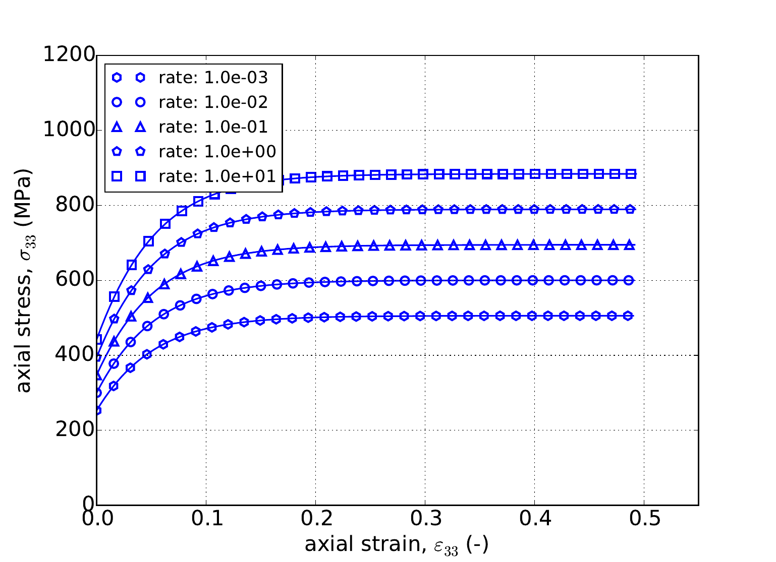
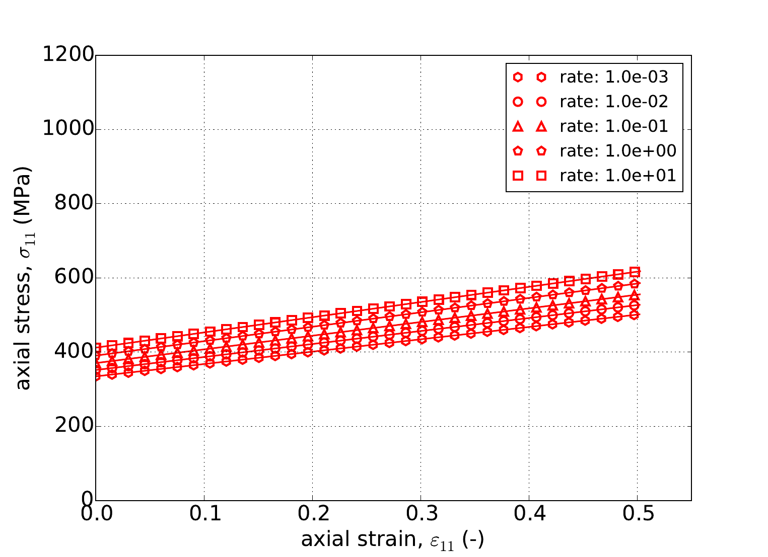
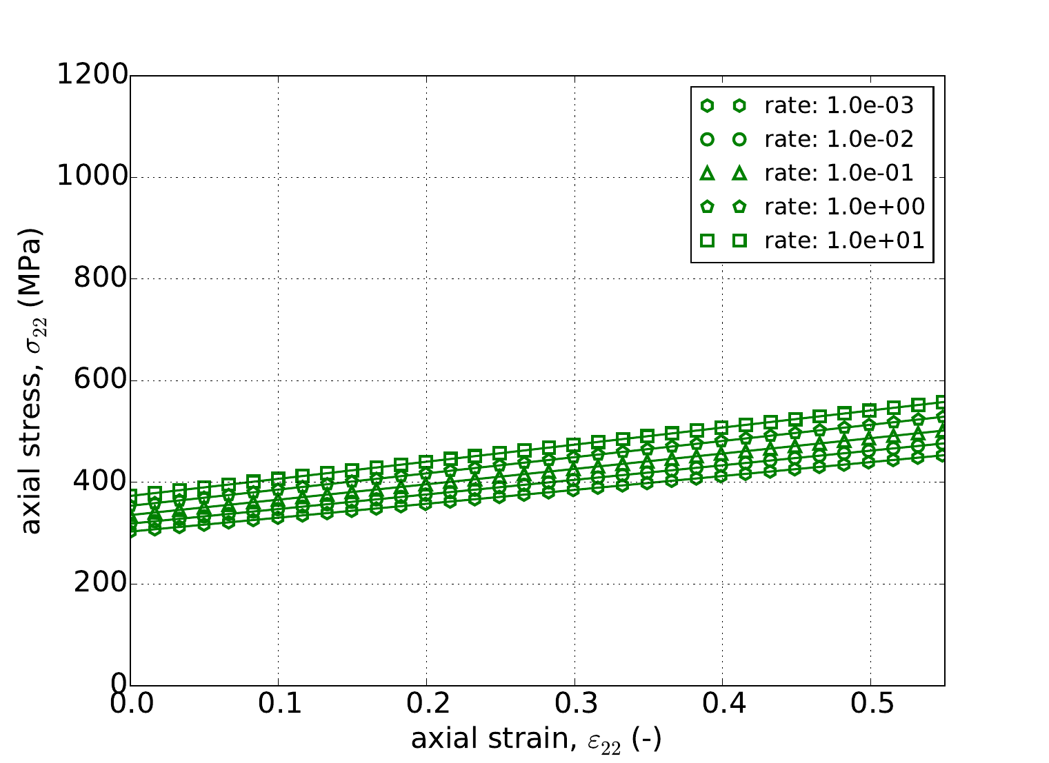
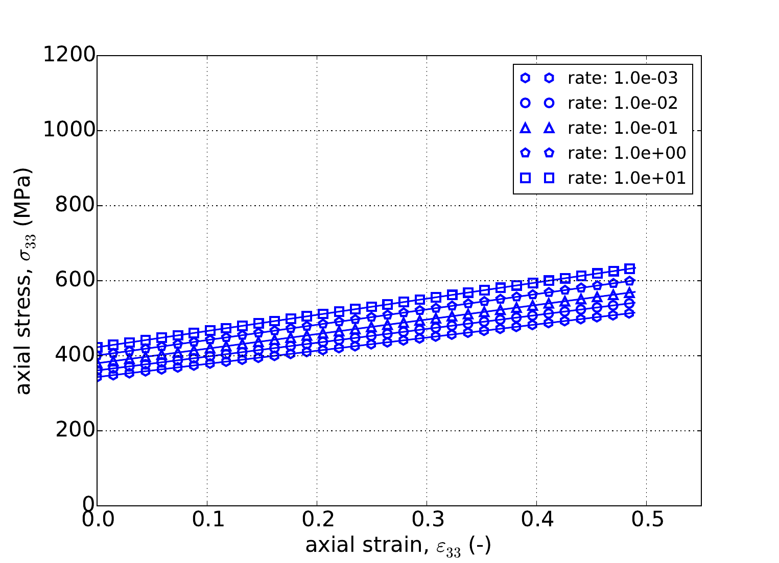
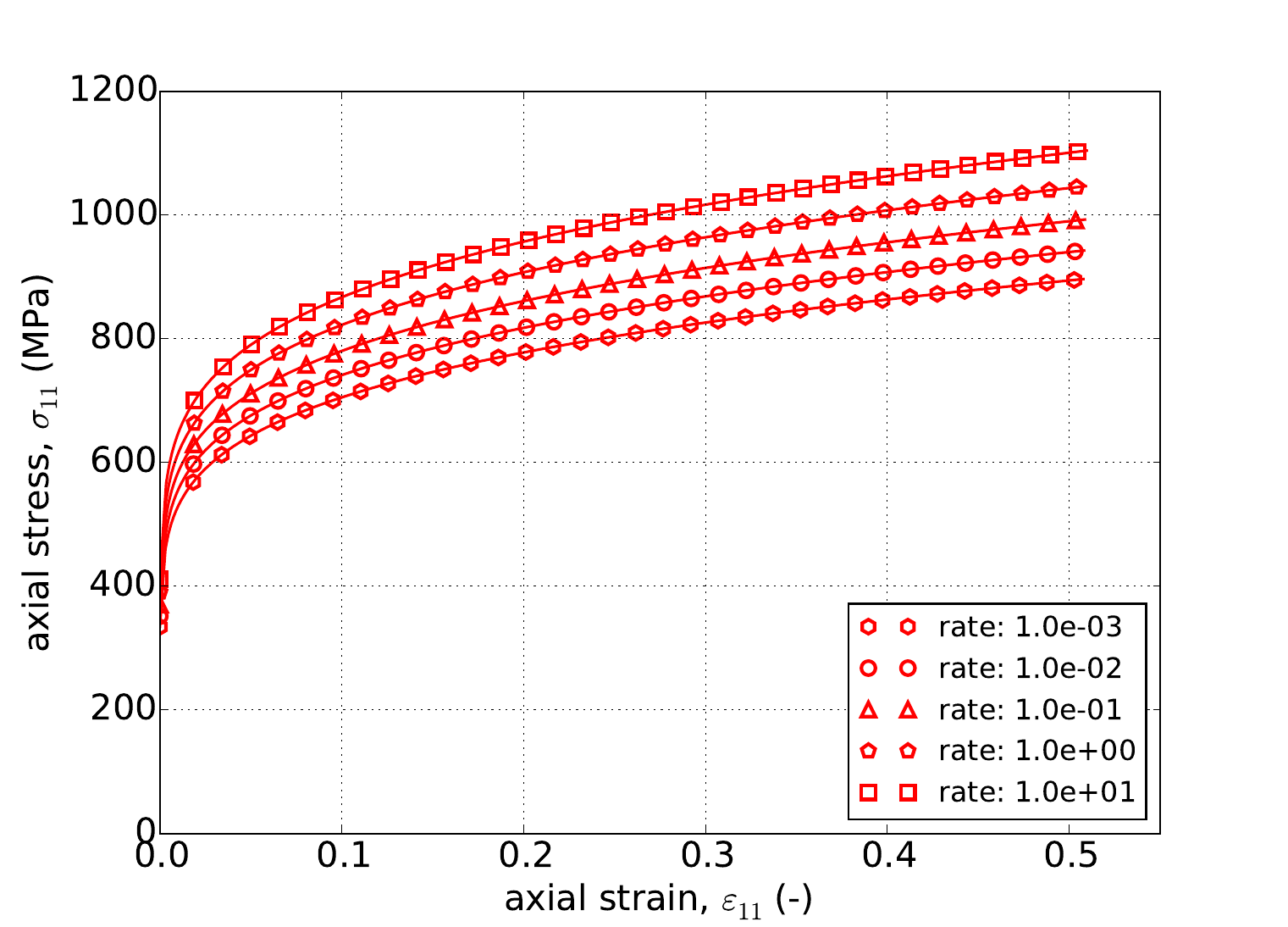
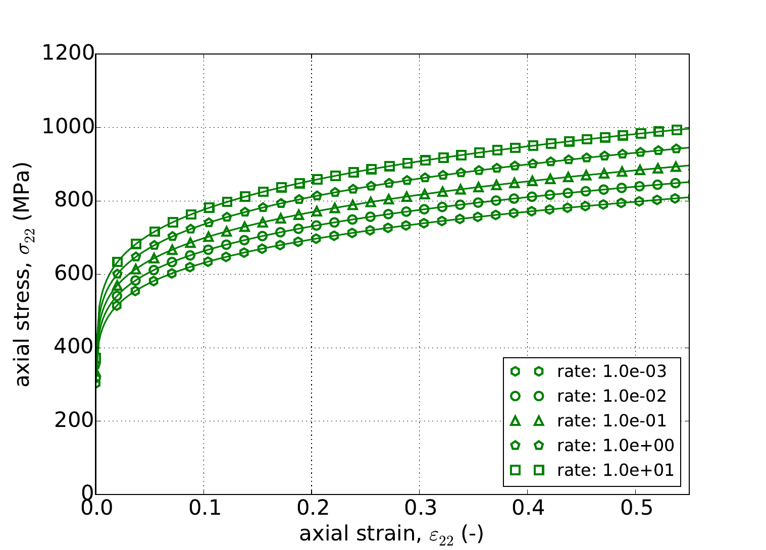
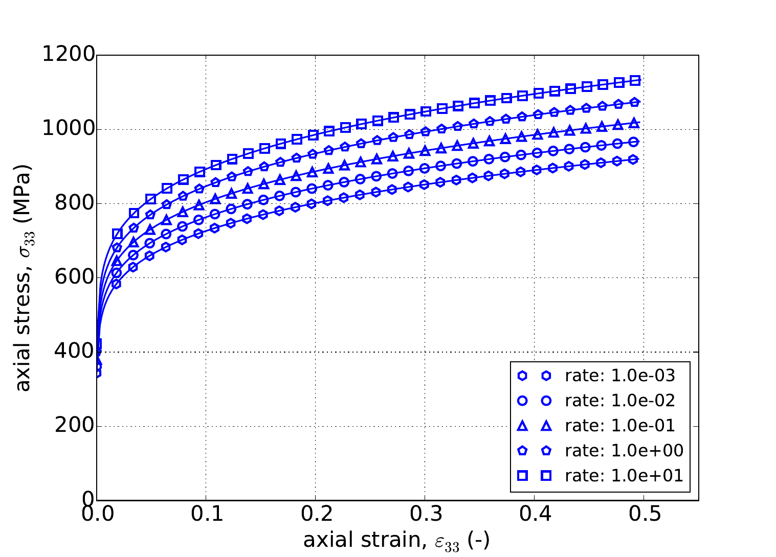
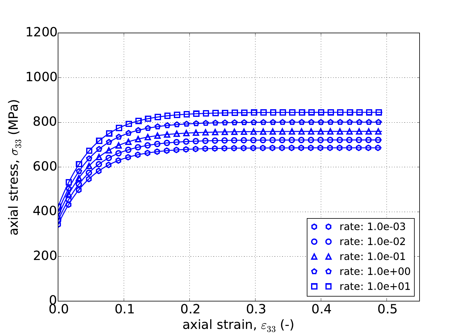
To investigate the uniaxial response of the Johnson-Cook rate dependent hardening model, the problem discussed in Appendix A is considered. In this analysis, the response depends only on time and the various \(c^{\prime}_i\) and \(c^{\prime\prime}_i\) Barlat yield surface coefficients. For a full-spectrum verification, forty-five different cases are evaluated using three different material principal directions (\(\hat{e}_1,~\hat{e}_2,\) and \(\hat{e}_3\)), five different rates (\(\dot{\bar{\varepsilon}}^p=~1\times10^{-3},~1\times10^{-2},~1\times10^{-1},~1\times10^{0}\) and \(1\times10^{1}~\text{s}^{-1}\)), and three different rate independent hardening models (linear, Voce, and power-law). All forty-five analytical and numerical results are presented in Fig. 4.84 and Fig. 4.85 and quite notable agreement is observed in each instance.
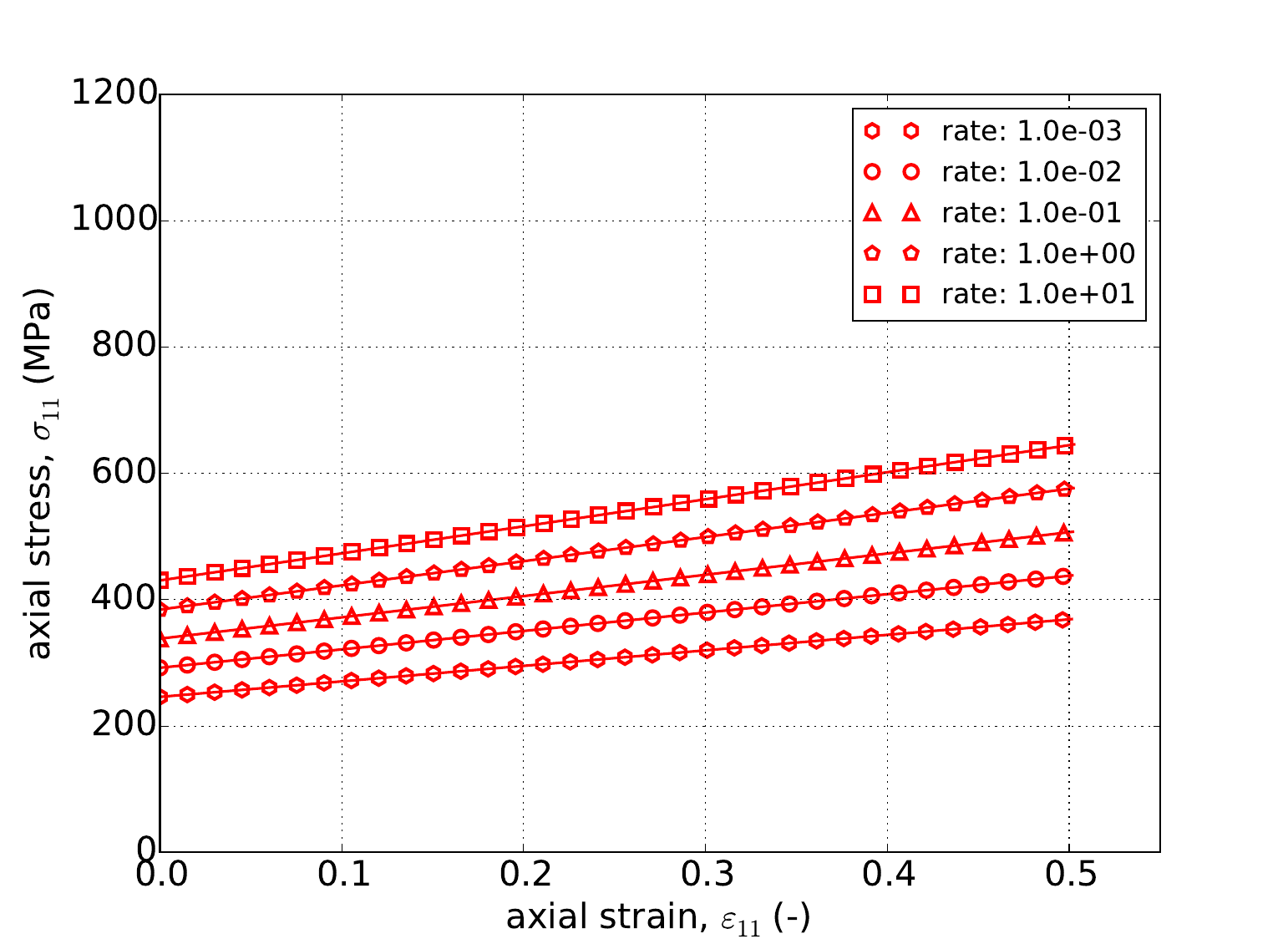 Linear Hardening -- 11
 Linear Hardening -- 22
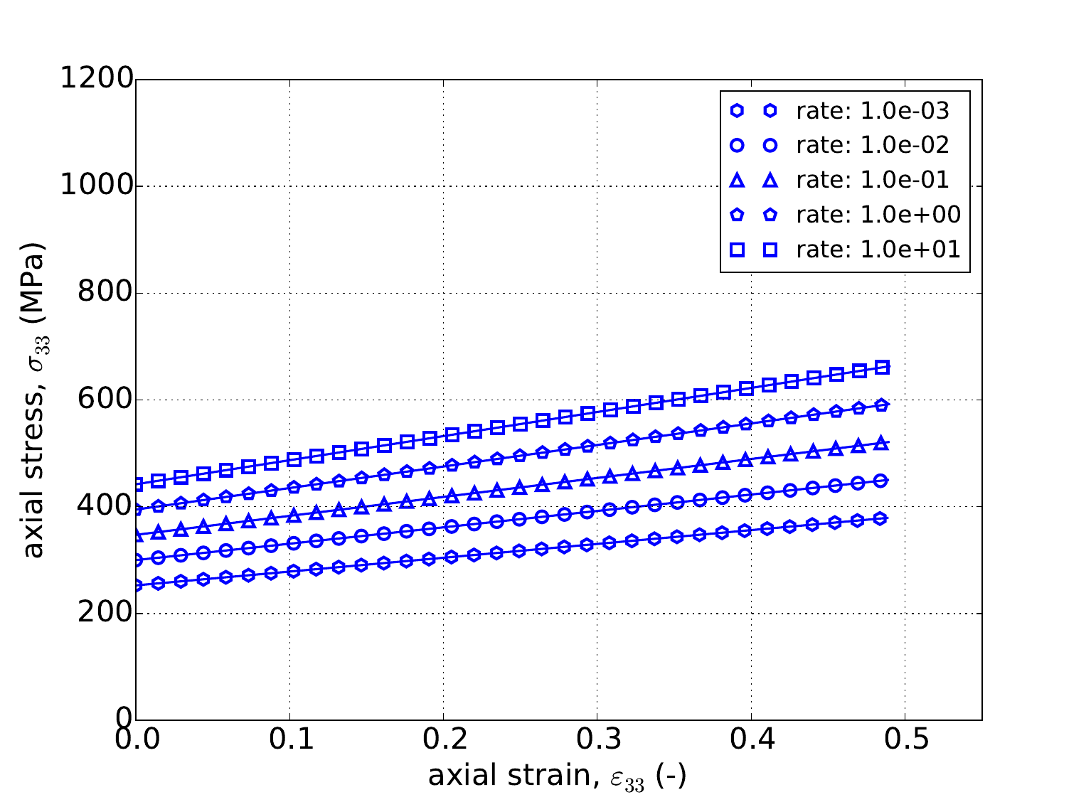 Linear Hardening -- 33
 Power-Law Hardening -- 11
 Power-Law Hardening -- 22
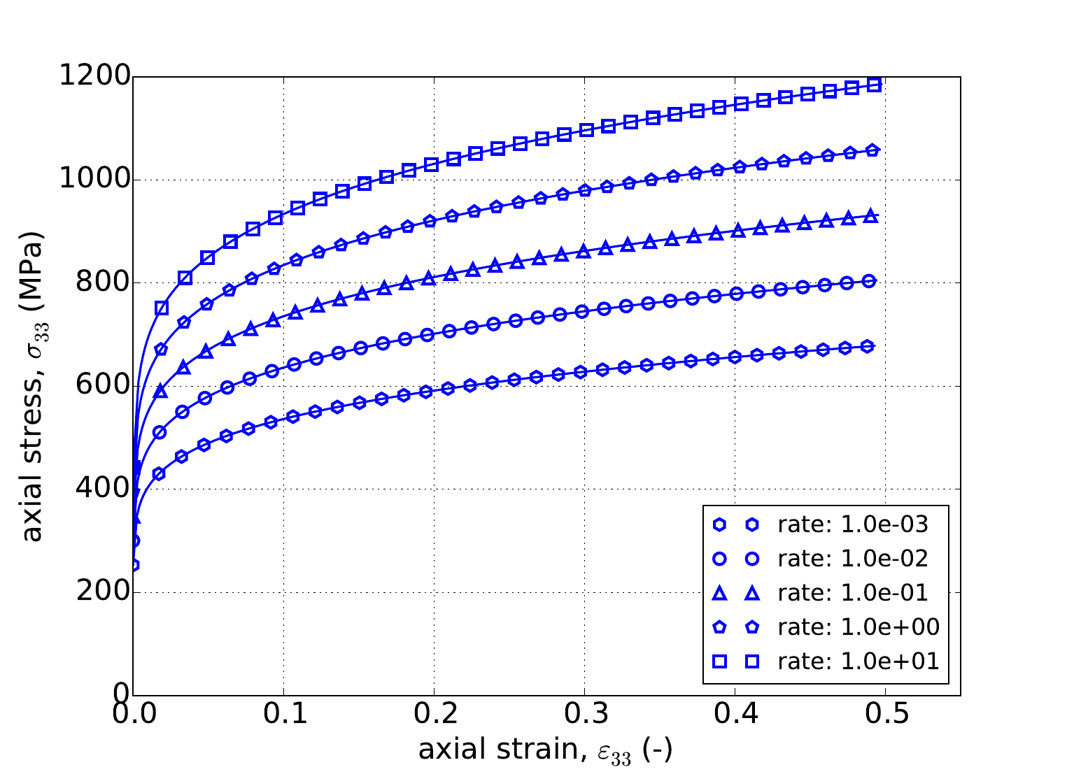 Power-Law Hardening -- 33
Fig. 4.84 Uniaxial stress-strain response of the Barlat plasticity model (\(a=8\)) with rate dependent, Johnson-Cook type hardening with (a-c) linear and (d-f) power-law rate independent hardening. Solid lines are analytical results while open symbols are numerical.
 Voce Hardening -- 11
 Voce Hardening -- 22
 Voce Hardening -- 33
Fig. 4.85 Uniaxial stress-strain response of the Barlat plasticity model (\(a=8\)) with rate dependent, Johnson-Cook type hardening with (a-c) Voce rate independent hardening. Solid lines are analytical results while open symbols are numerical.
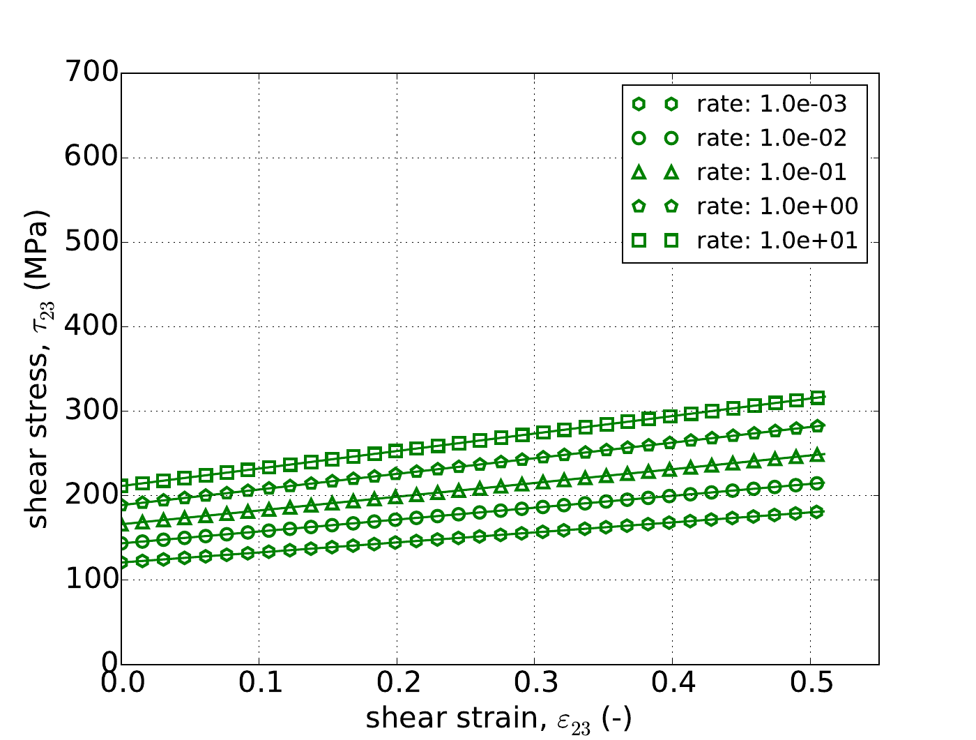
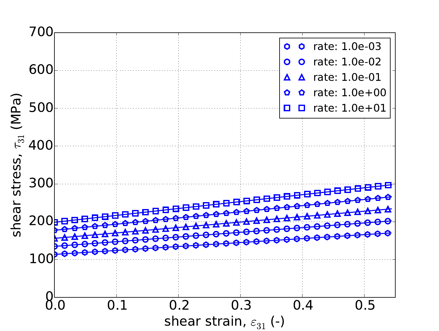
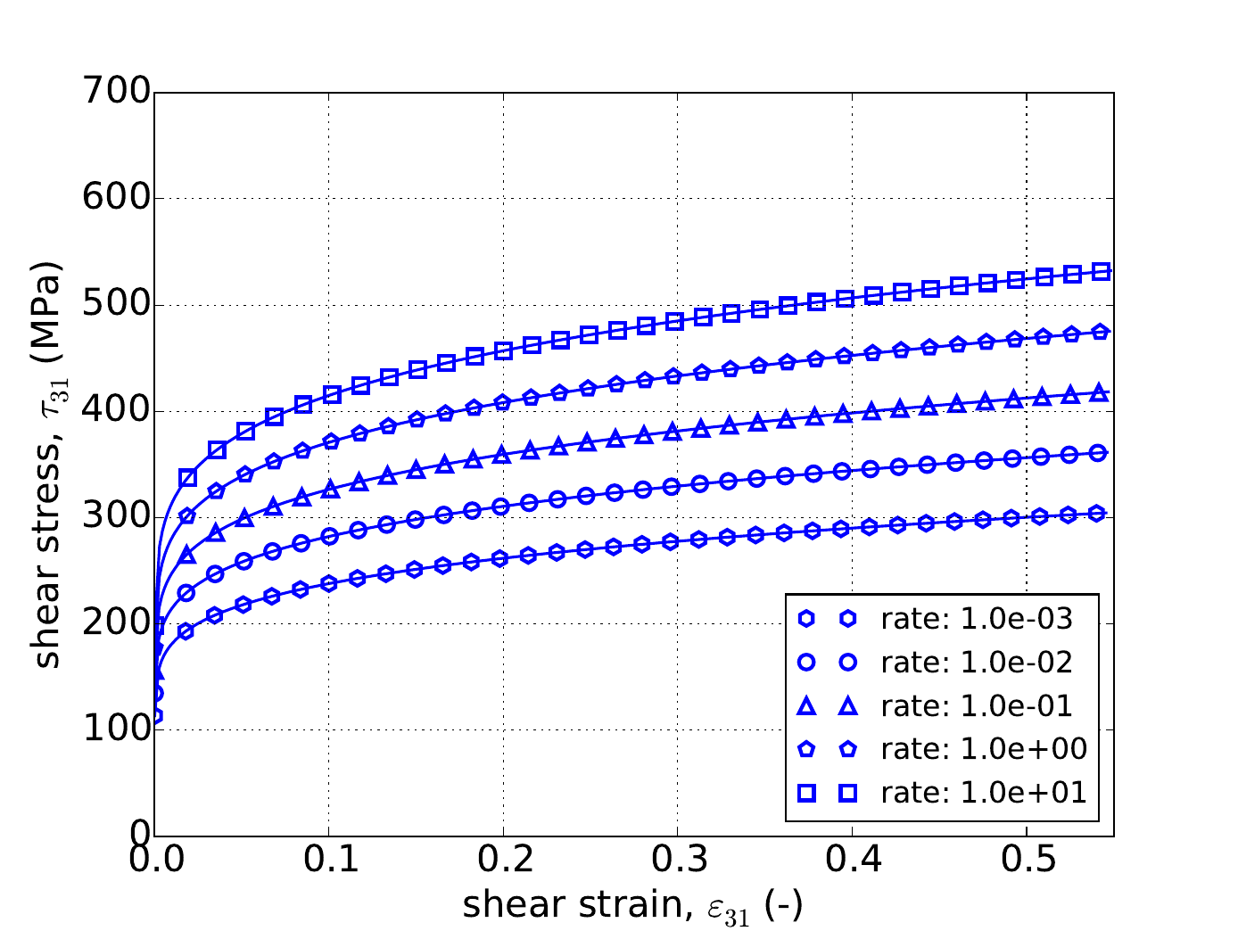
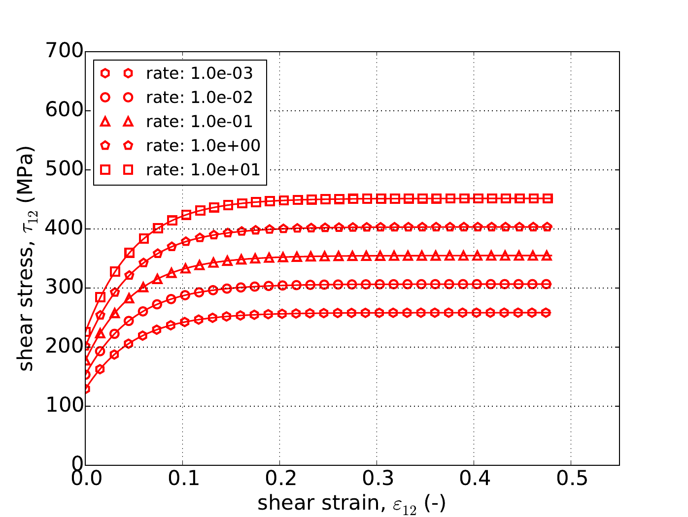
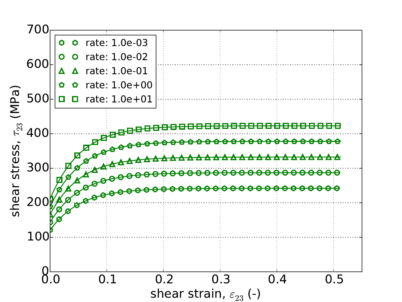
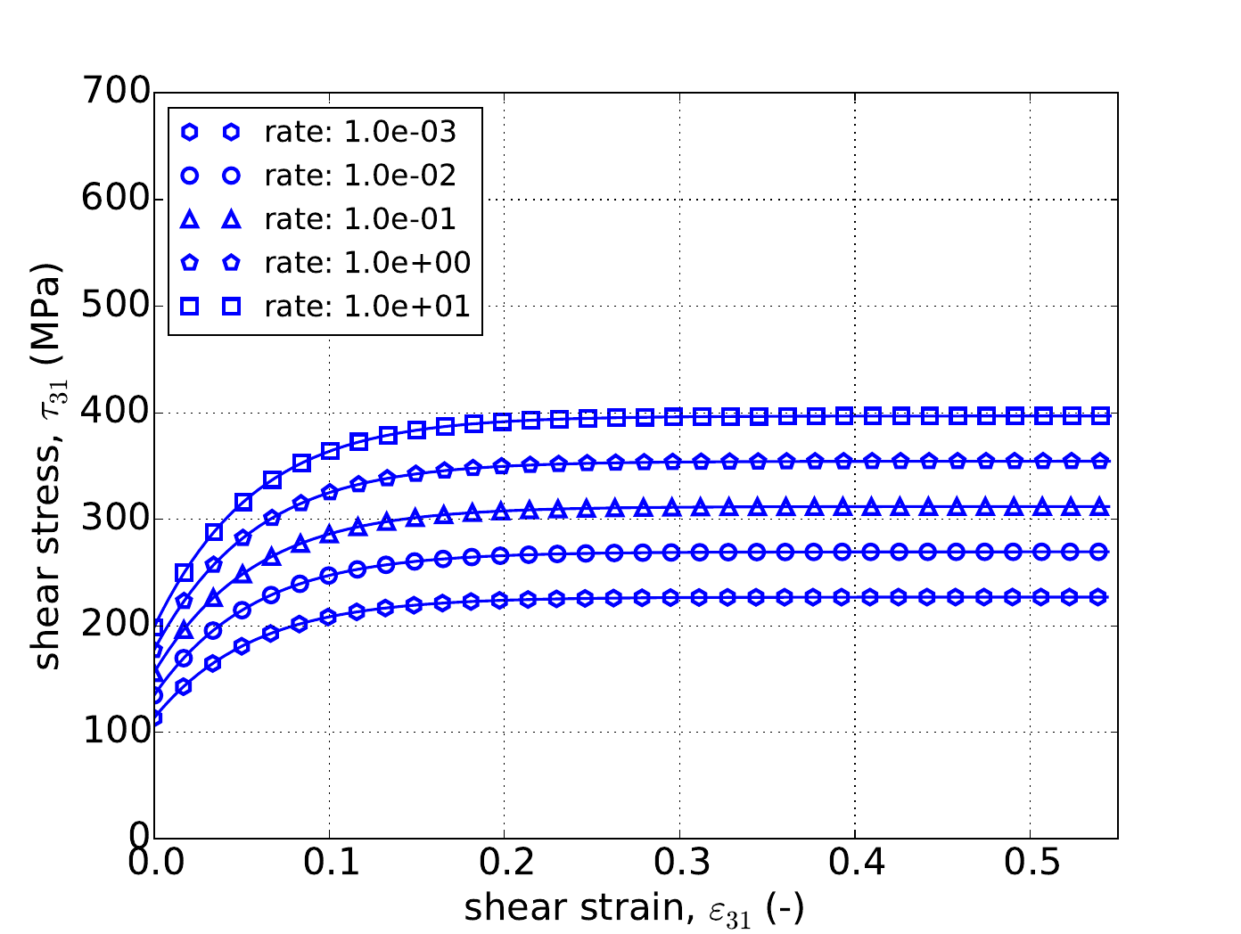
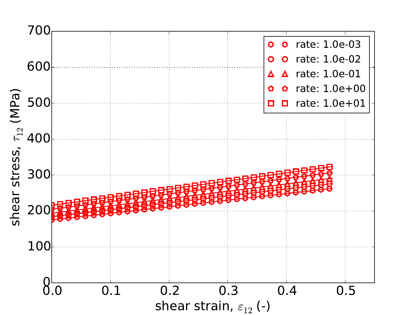
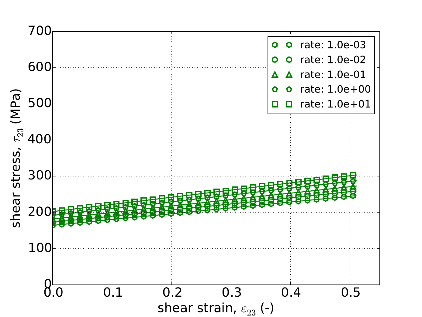
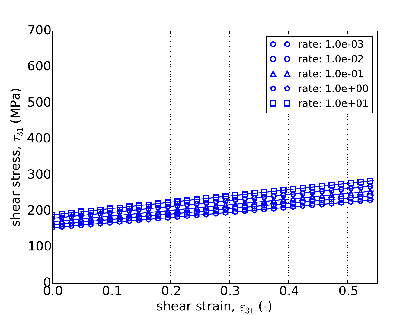
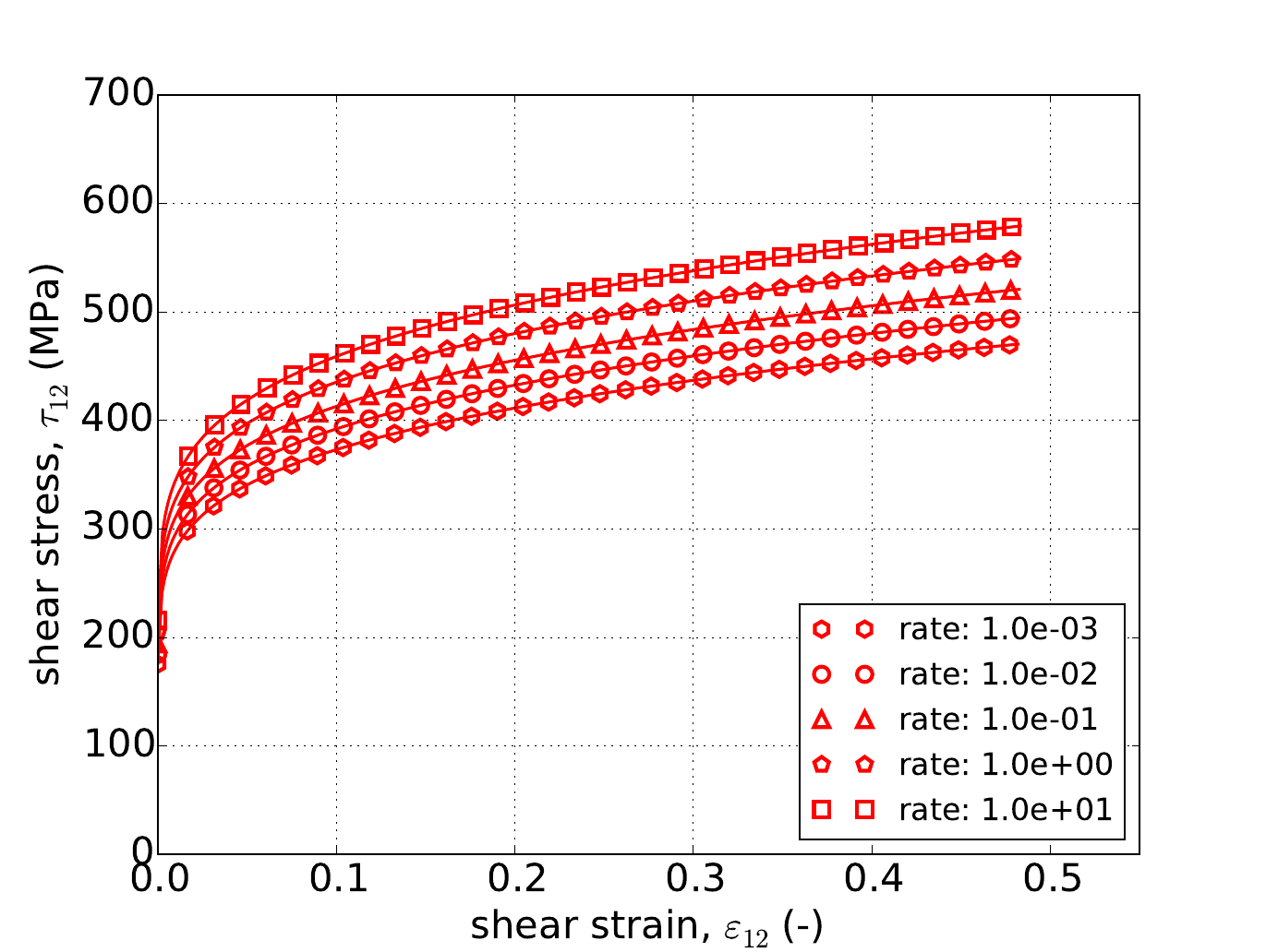
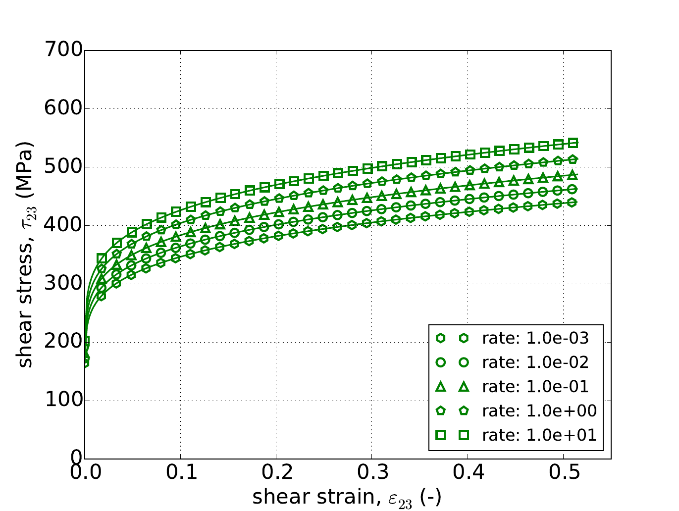
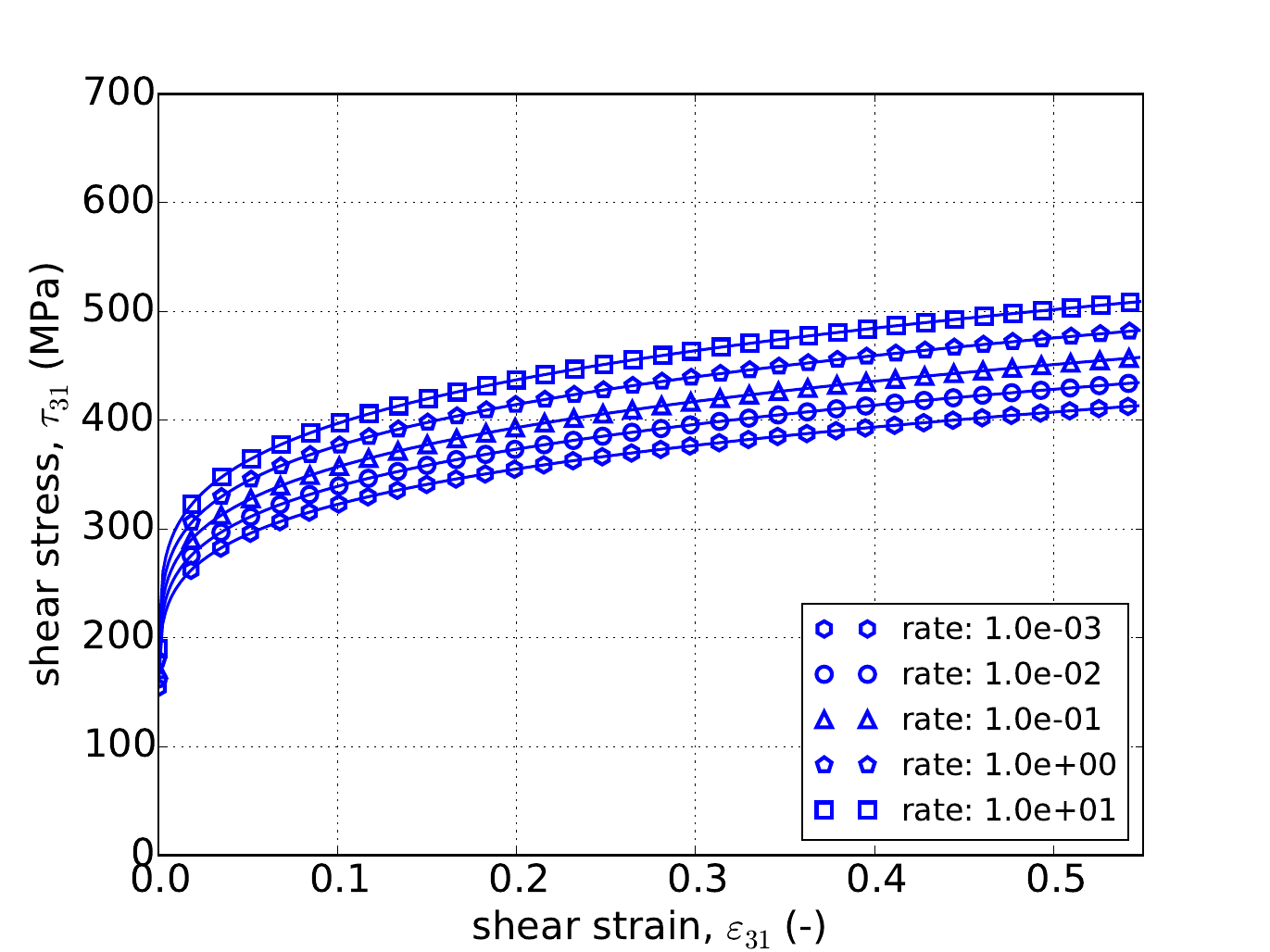
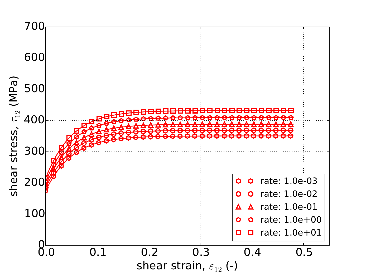
For the pure shear case, the forty-five different permutations are again explored. The same five rates and three hardening models are used although three different shearing planes are used instead of the three principal directions. The solution of the pure shear problem is described in Appendix A and the analytical and numerical results are presented in Fig. 4.86 and Fig. 4.87. As with the uniaxial stress response excellent correspondence is noted between the two sets of results.
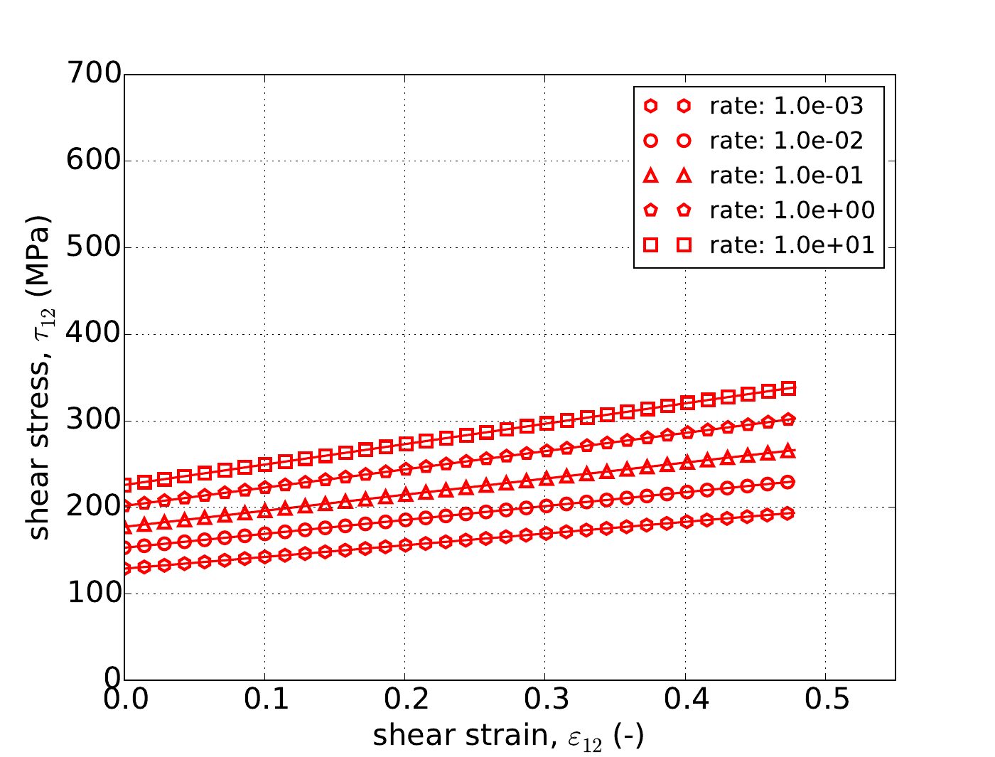 Linear Hardening -- 11
 Linear Hardening -- 22
 Linear Hardening -- 33
 Power-Law Hardening -- 11
 Power-Law Hardening -- 22
 Power-Law Hardening -- 33
Fig. 4.86 Stress-strain response of the Barlat plasticity model (\(a=8\)) with rate dependent, Johnson-Cook type hardening in pure shear with (a-c) linear and (d-f) power-law rate independent hardening. Solid lines are analytical results while open symbols are numerical.
 Voce Hardening -- 11
 Voce Hardening -- 22
 Voce Hardening -- 33
Fig. 4.87 Stress-strain response of the Barlat plasticity model (\(a=8\)) with rate dependent, Johnson-Cook type hardening in pure shear with (a-c) Voce rate independent hardening. Solid lines are analytical results while open symbols are numerical.
4.16.3.3.5. Power-Law Breakdown
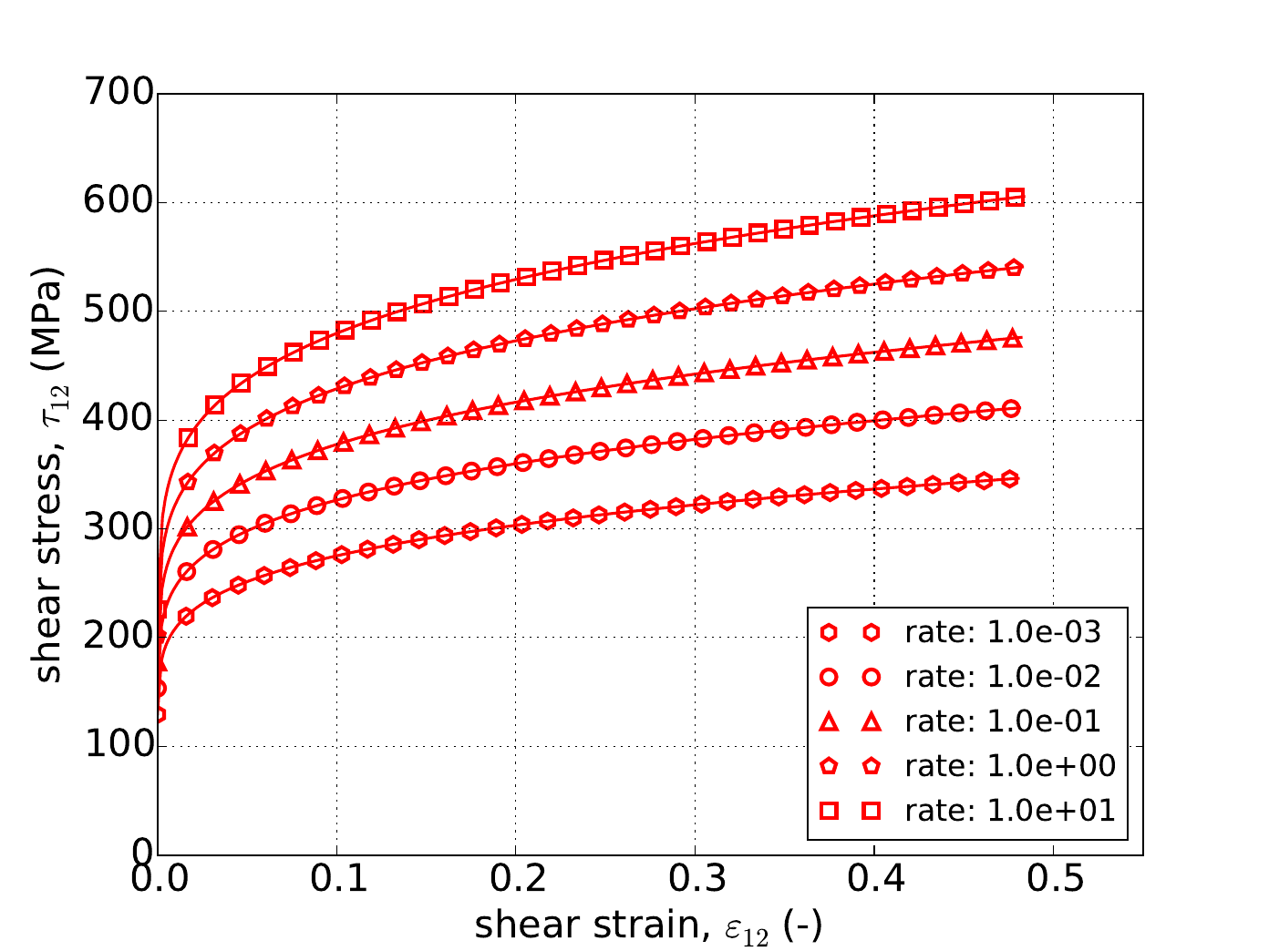
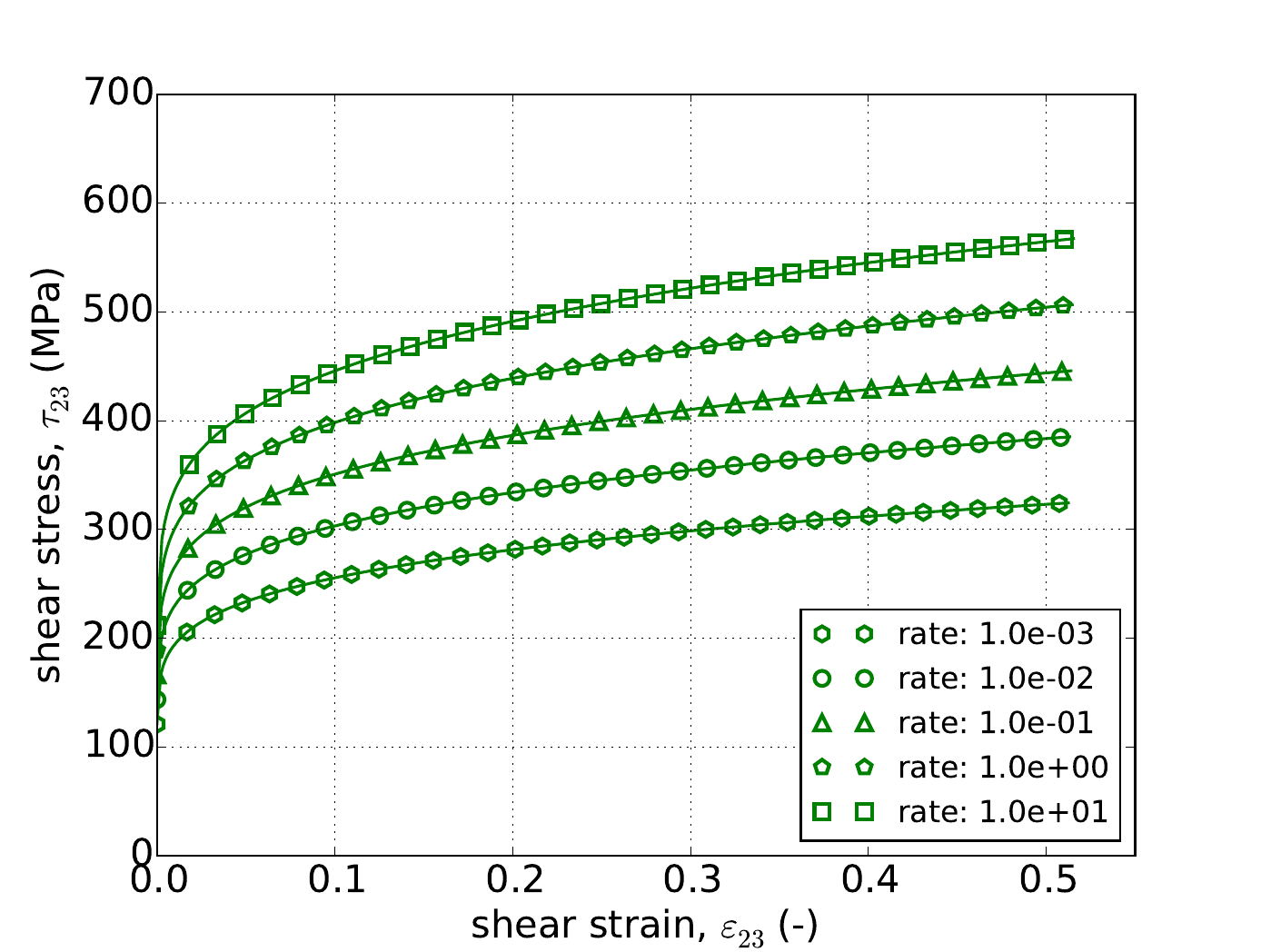
In the case of the power-law Breakdown model, verification is again pursued through the problem of Appendix A and using the same forty-five cases discussed with the Johnson-Cook model. Corresponding results are given in Fig. 4.88 and Fig. 4.89 and as with the preceding results substantial convergence is noted between the analytical and numerical results giving further credence to the hardening models.
 Linear Hardening -- 11
 Linear Hardening -- 22
 Linear Hardening -- 33
 Power-Law Hardening -- 11
 Power-Law Hardening -- 22
 Power-Law Hardening -- 33
Fig. 4.88 Uniaxial stress-strain response of the Barlat plasticity model (\(a=8\)) with rate dependent, power-law breakdown type hardening with (a-c) linear and (d-f) power-law rate independent hardening. Solid lines are analytical while open symbols are numerical.
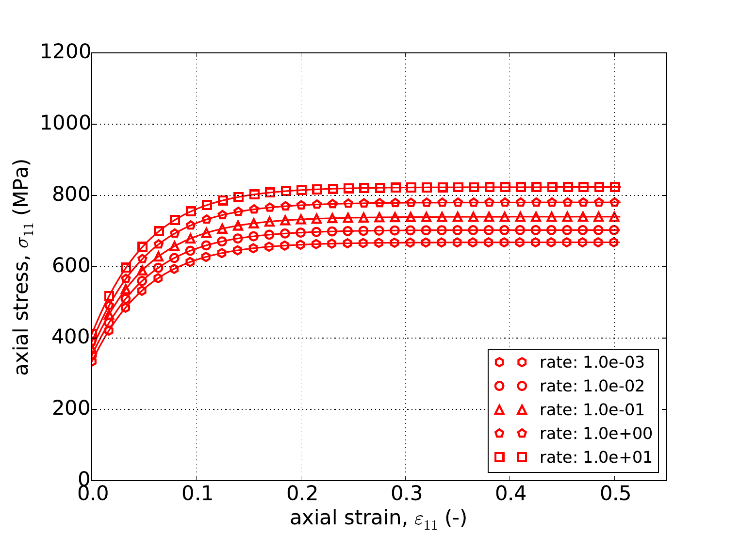 Voce Hardening -- 11
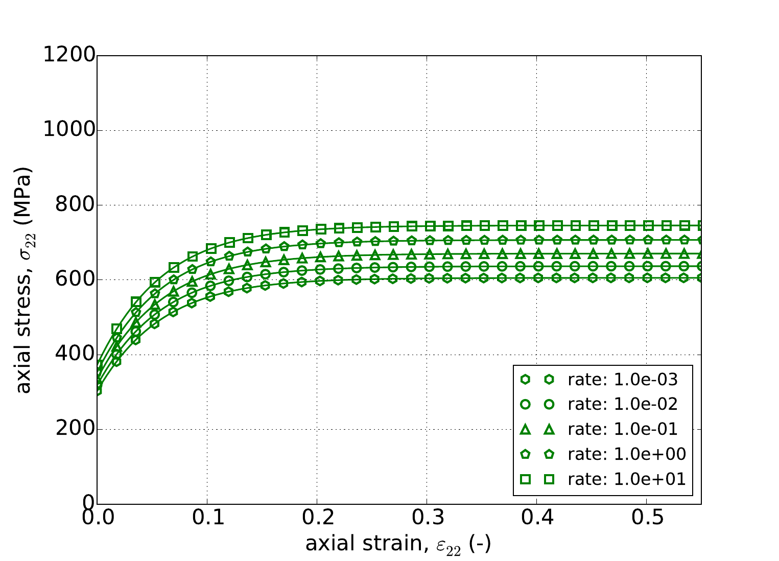 Voce Hardening -- 22
 Voce Hardening -- 33
Fig. 4.89 Uniaxial stress-strain response of the Barlat plasticity model (\(a=8\)) with rate dependent, power-law breakdown type hardening with (a-c) Voce rate independent hardening. Solid lines are analytical while open symbols are numerical.
As with the uniaxial stress case, the pure shear capabilities are interrogated through the procedure of Appendix A using the same forty-five cases outlined in the Johnson-Cook discussion. The analytical and numerical results are presented in Fig. 4.90 and Fig. 4.91. Again, the two result sets align beautifully enabling further capability credibility.
 Linear Hardening -- 11
 Linear Hardening -- 22
 Linear Hardening -- 33
 Power-Law Hardening -- 11
 Power-Law Hardening -- 22
 Power-Law Hardening -- 33
Fig. 4.90 Stress-strain response of the Barlat plasticity model (\(a=8\)) with rate dependent, power-law breakdown type hardening in pure shear with (a-c) linear and (d-f) power-law rate independent hardening. Solid lines are analytical results while open symbols are numerical.
 Voce Hardening -- 11
 Voce Hardening -- 22
 Voce Hardening -- 33
Fig. 4.91 Stress-strain response of the Barlat plasticity model (\(a=8\)) with rate dependent, power-law breakdown type hardening in pure shear with (a-c) Voce rate independent hardening. Solid lines are analytical results while open symbols are numerical.
4.16.4. User Guide
BEGIN PARAMETERS FOR MODEL BARLAT_PLASTICITY
  #
  # Elastic constants
  #
  YOUNGS MODULUS = <real>
  POISSONS RATIO = <real>
  SHEAR MODULUS  = <real>
  BULK MODULUS   = <real>
  LAMBDA         = <real>
  TWO MU         = <real>
  #
  # Material coordinates system definition
  #
  COORDINATE SYSTEM             = <string> coordinate_system_name
  DIRECTION FOR ROTATION        = <real> 1|2|3
  ALPHA                         = <real> (degrees)
  SECOND DIRECTION FOR ROTATION = <real> 1|2|3
  SECOND ALPHA                  = <real> (degrees)
  #
  # Yield surface parameters
  #
  YIELD STRESS = <real>
  A            = <real> (4.0)
  CP12         = <real> (1.0)
  CP13         = <real> (1.0)
  CP21         = <real> (1.0)
  CP23         = <real> (1.0)
  CP31         = <real> (1.0)
  CP32         = <real> (1.0)
  CP44         = <real> (1.0)
  CP55         = <real> (1.0)
  CP66         = <real> (1.0)
  CPP12        = <real> (1.0)
  CPP13        = <real> (1.0)
  CPP21        = <real> (1.0)
  CPP23        = <real> (1.0)
  CPP31        = <real> (1.0)
  CPP32        = <real> (1.0)
  CPP44        = <real> (1.0)
  CPP55        = <real> (1.0)
  CPP66        = <real> (1.0)
#
  #
  # Hardening model
  #
  HARDENING MODEL = LINEAR | POWER_LAW | VOCE | USER_DEFINED |
  FLOW_STRESS | DECOUPLED_FLOW_STRESS | JOHNSON_COOK |
  POWER_LAW_BREAKDOWN
  #
  # Linear hardening
  #
  HARDENING MODULUS = <real>
  #
  # Power-law hardening
  #
  HARDENING CONSTANT = <real>
  HARDENING EXPONENT = <real> (0.5)
  LUDERS STRAIN      = <real> (0.0)
  #
  # Voce hardening
  #
  HARDENING MODULUS       = <real>
  EXPONENTIAL COEFFICIENT = <real>
  #
  # Johnson-Cook hardening
  #
  HARDENING FUNCTION = <string>hardening_function_name
  RATE CONSTANT      = <real>
  REFERENCE RATE     = <real>
  #
  # Power law breakdown hardening
  #
  HARDENING FUNCTION = <string>hardening_function_name
  RATE COEFFICIENT   = <real>
  RATE EXPONENT      = <real>
  # User defined hardening
  #
  HARDENING FUNCTION = <string>hardening_function_name
  #
#
  #
  # Following Commands Pertain to Flow_Stress Hardening Model
  #
  #    -  Isotropic Hardening model
  #
  ISOTROPIC HARDENING MODEL = LINEAR | POWER_LAW | VOCE |
                              USER_DEFINED
  #
  # Specifications for Linear, Power-law, and Voce same as above
  #
  # User defined hardening
  #
  ISOTROPIC HARDENING FUNCTION = <string>iso_hardening_fun_name
  #
  #     - Rate dependence
  #
  RATE MULTIPLIER = JOHNSON_COOK | POWER_LAW_BREAKDOWN |
     USER_DEFINED | RATE_INDEPENDENT (RATE_INDEPENDENT)
  #
  # Specifications for Johnson-Cook, Power-law-breakdown
  #     same as before EXCEPT no need to specify a
  #     hardening function
  #
  # User defined rate multiplier
  #
  RATE MULTIPLIER FUNCTION = <string> rate_mult_function_name
  #
  #     - Temperature dependence
  #
  TEMPERATURE MULTIPLIER = JOHNSON_COOK | USER_DEFINED |
     TEMPERATURE_INDEPENDENT (TEMPERATURE_INDEPENDENT)
  #
  #  Johnson-Cook temperature dependence
  #
  MELTING TEMPERATURE   = <real>
  REFERENCE TEMPERATURE = <real>
  TEMPERATURE EXPONENT  = <real>
  #
  #  User-defined temperature dependence
  TEMPERATURE MULTIPLIER FUNCTION = <string>temp_mult_function_name
  #
  # Following Commands Pertain to Decoupled_Flow_Stress Hardening Model
  #
  #    -  Isotropic Hardening model
  #
  ISOTROPIC HARDENING MODEL = LINEAR | POWER_LAW | VOCE | USER_DEFINED
  #
  # Specifications for Linear, Power-law, and Voce same as above
  #
  # User defined hardening
  #
  ISOTROPIC HARDENING FUNCTION = <string>isotropic_hardening_function_name
  #
  #     - Rate dependence
  #
  YIELD RATE MULTIPLIER = JOHNSON_COOK | POWER_LAW_BREAKDOWN |
              USER_DEFINED | RATE_INDEPENDENT (RATE_INDEPENDENT)
  #
  # Specifications for Johnson-Cook, Power-law-breakdown same as before
  #     EXCEPT no need to specify a hardening function
  #     AND should be preceded by YIELD
  #
  #     As an example for Johnson-Cook yield rate dependence,
  #
  YIELD RATE CONSTANT  = <real>
  YIELD REFERENCE RATE = <real>
  #
  # User defined rate multiplier
  #
  YIELD RATE MULTIPLIER FUNCTION = <string>yield_rate_mult_function_name
  #
  HARDENING_RATE MULTIPLIER = JOHNSON_COOK | POWER_LAW_BREAKDOWN |
              USER_DEFINED | RATE_INDEPENDENT (RATE_INDEPENDENT)
  #
  #     Syntax same as for yield parameters but with a HARDENING prefix
  #
  #     - Temperature dependence
  #
  YIELD TEMPERATURE MULTIPLIER = JOHNSON_COOK | USER_DEFINED |
            TEMPERATURE_INDEPENDENT (TEMPERATURE_INDEPENDENT)
  #
  #  Johnson-Cook temperature dependence
  #
  YIELD MELTING TEMPERATURE   = <real>
  YIELD REFERENCE TEMPERATURE = <real>
  YIELD TEMPERATURE EXPONENT  = <real>
  #
  #  User-defined temperature dependence
  YIELD TEMPERATURE MULTIPLIER FUNCTION = <string>yield_temp_mult_fun_name
  #
  HARDENING TEMPERATURE MULTIPLIER = JOHNSON_COOK | USER_DEFINED |
            TEMPERATURE_INDEPENDENT (TEMPERATURE_INDEPENDENT)
  #
  #   Syntax for hardening constants same as for yield but
  #            with HARDENING prefix
#
  #
  # Optional Failure Definitions
  #    Following only need to be defined if intend to use failure model
  #
  FAILURE MODEL = TEARING_PARAMETER | JOHNSON_COOK_FAILURE | WILKINS
                  | MODULAR_FAILURE | MODULAR_BCJ_FAILURE

  CRITICAL FAILURE PARAMETER = <real>
  #
  # TEARING_PARAMETER Failure model definitions
  #
  TEARING PARAMETER EXPONENT = <real>
  #
  # JOHNSON_COOK_FAILURE Failure model definitions
  #
  JOHNSON COOK D1       = <real>
  JOHNSON COOK D2       = <real>
  JOHNSON COOK D3       = <real>
  JOHNSON COOK D4       = <real>
  JOHNSON COOK D5       = <real>
  #
  #Following Johnson-Cook parameters can only be defined once.  As such, only
  #  needed if not previously defined via Johnson-Cook multipliers
  #  w/ flow-stress hardening.  Does need to be defined
  #  w/ Decoupled Flow Stress
  #
  REFERENCE RATE        = <real>
  REFERENCE TEMPERATURE = <real>
  MELTING TEMPERATURE   = <real>
  #
  # WILKINS Failure model definitions
  #
  WILKINS ALPHA    = <real>
  WILKINS BETA     = <real>
  WILKINS PRESSURE = <real>
  #
  #  MODULAR_FAILURE Failure model definitions
  #
  PRESSURE MULTIPLIER         = PRESSURE_INDEPENDENT | WILKINS
                                | USER_DEFINED (PRESSURE_INDEPENDENT)
  LODE ANGLE MULTIPLIER       = LODE_ANGLE_INDEPENDENT |
                                WILKINS (LODE_ANGLE_INDEPENDENT)
  TRIAXIALITY MULTIPLIER      = TRIAXIALITY_INDEPENDENT | JOHNSON_COOK
                                | USER_DEFINED (TRIAXIALITY_INDEPENDENT)
  RATE FAIL MULTIPLIER        = RATE_INDEPENDENT | JOHNSON_COOK
                                | USER_DEFINED (RATE_INDEPENDENT)
  TEMPERATURE FAIL MULTIPLIER = TEMPERATURE_INDEPENDENT | JOHNSON_COOK
                                | USER_DEFINED (TEMPERATURE_INDEPENDENT)
  #
  # Individual multiplier definitions
  #
  PRESSURE MULTIPLIER = WILKINS
  WILKINS ALPHA       = <real>
  WILKINS PRESSURE    = <real>
  #
  PRESSURE MULTIPLIER = USER_DEFINED
  PRESSURE MULTIPLIER FUNCTION = <string> pressure_multiplier_fun_name
  #
  LODE ANGLE MULTIPLIER = WILKINS
  WILKINS BETA          = <real>
  #
  TRIAXIALITY MULTIPLIER = JOHNSON_COOK
  JOHNSON COOK D1        = <real>
  JOHNSON COOK D2        = <real>
  JOHNSON COOK D3        = <real>
  #
  TRIAXIALITY MULTIPLIER = USER_DEFINED
  TRIAXIALITY MULTIPLIER FUNCTION = <string> triaxiality_multiplier_fun_name
  #
  RATE FAIL MULTIPLIER = JOHNSON_COOK
  JOHNSON COOK D4      = <real>
  # REFERENCE RATE should only be added if not previously defined
  REFERENCE RATE       = <real>
  #
  RATE FAIL MULTIPLIER = USER_DEFINED
  RATE FAIL MULTIPLIER FUNCTION = <string> rate_fail_multiplier_fun_name
  #
  TEMPERATURE FAIL MULTIPLIER = JOHNSON_COOK
  JOHNSON COOK D5             = <real>
  # JC Temperatures should only be defined if not previously given
  REFERENCE TEMPERATURE       = <real>
  MELTING TEMPERATURE         = <real>
  #
  TEMPERATURE FAIL MULTIPLIER          = USER_DEFINED
  TEMPERATURE FAIL MULTIPLIER FUNCTION = <string> temp_multiplier_fun_name
  #
  # MODULAR_BCJ_FAILURE Failure model definitions
  #
  INITIAL DAMAGE    = <real>
  INITIAL VOID SIZE = <real>
  DAMAGE BETA       = <real> (0.5)
  GROWTH MODEL      = COCKS_ASHBY | NO_GROWTH (NO_GROWTH)
  NUCLEATION MODEL  = HORSTEMEYER_GOKHALE | CHU_NEEDLEMAN_STRAIN
                      | NO_NUCLEATION (NO_NUCLEATION)
  #
  GROWTH RATE FAIL MULTIPLIER        = JOHNSON_COOK | USER_DEFINED
                                       | RATE_INDEPENDENT
                                       (RATE_INDEPENDENT)
  GROWTH TEMPERATURE FAIL MULTIPLIER = JOHNSON_COOK | USER_DEFINED
                                       | TEMPERATURE_INDEPENDENT
                                       (TEMPERATURE_INDEPENDENT)
  #
  NUCLEATION RATE FAIL MULTIPLIER        = JOHNSON_COOK | USER_DEFINED
                                           | RATE_INDEPENDENT
                                           (RATE_INDEPENDENT)
  NUCLEATION TEMPERATURE FAIL MULTIPLIER = JOHNSON_COOK | USER_DEFINED
                                           | TEMPERATURE_INDEPENDENT
                                           (TEMPERATURE_INDEPENDENT)
  #
  # Definitions for individual growth and nucleation models
  #
  GROWTH MODEL = COCKS_ASHBY
  DAMAGE EXPONENT = <real> (0.5)
  #
  NUCLEATION MODEL      = HORSTEMEYER_GOKHALE
  NUCLEATION PARAMETER1 = <real> (0.0)
  NUCLEATION PARAMETER2 = <real> (0.0)
  NUCLEATION PARAMETER3 = <real> (0.0)
  #
  NUCLEATION MODEL          = CHU_NEEDLEMAN_STRAIN
  NUCLEATION AMPLITUDE      = <real>
  MEAN NUCLEATION STRAIN    = <real>
  NUCLEATION STRAIN STD DEV = <real>
  #
  # Definitions for rate and temperature fail multiplier
  #   Note: only showing definitions for growth.
  #    Nucleation terms are the same just with NUCLEATION instead
  #    of GROWTH
  #
  GROWTH RATE FAIL MULTIPLIER = JOHNSON_COOK
  GROWTH JOHNSON COOK D4      = <real>
  GROWTH REFERENCE RATE       = <real>
  #
  GROWTH RATE FAIL MULTIPLIER          = USER_DEFINED
  GROWTH RATE FAIL MULTIPLIER FUNCTION = <string> growth_rate_fail_mult_func
  #
  GROWTH TEMPERATURE FAIL MULTIPLIER = JOHNSON_COOK
  GROWTH JOHNSON COOK D5             = <real>
  GROWTH REFERENCE TEMPERATURE       = <real>
  GROWTH MELTING TEMPERATURE         = <real>
  #
  GROWTH TEMPERATURE FAIL MULTIPLIER          = USER_DEFINED
  GROWTH TEMPERATURE FAIL MULTIPLIER FUNCTION = <string> temp_fail_mult_func
  #
#
  #
  # Optional Adiabatic Heating/Thermal Softening  Definitions
  #    Following only need to be defined if intend to use failure model
  #
  THERMAL SOFTENING MODEL = ADIABATIC | COUPLED
  #
  SPECIFIC HEAT = <real> # not needed for COUPLED
  BETA_TQ       = <real>
END [PARAMETERS FOR MODEL BARLAT_PLASTICITY]
In the command blocks that define the Barlat plasticity model:
The reference nominal yield stress, \(\bar{\sigma}\), is defined with the
YIELD STRESScommand line.The exponent for the yield surface description, \(a\), is defined with the
Acommand line.The transformation coefficient, \(c^{'}_{12}\), is defined with the
CP12command line. It is defaulted to 1.0.The transformation coefficient, \(c^{'}_{13}\), is defined with the
CP13command line. It is defaulted to 1.0.The transformation coefficient, \(c^{'}_{21}\), is defined with the
CP21command line. It is defaulted to 1.0.The transformation coefficient, \(c^{'}_{23}\), is defined with the
CP23command line. It is defaulted to 1.0.The transformation coefficient, \(c^{'}_{31}\), is defined with the
CP31command line. It is defaulted to 1.0.The transformation coefficient, \(c^{'}_{32}\), is defined with the
CP32command line. It is defaulted to 1.0.The transformation coefficient, \(c^{'}_{44}\), is defined with the
CP44command line. It is defaulted to 1.0.The transformation coefficient, \(c^{'}_{55}\), is defined with the
CP55command line. It is defaulted to 1.0.The transformation coefficient, \(c^{'}_{66}\), is defined with the
CP66command line. It is defaulted to 1.0.The transformation coefficient, \(c^{''}_{12}\), is defined with the
CPP12command line. It is defaulted to 1.0.The transformation coefficient, \(c^{''}_{13}\), is defined with the
CPP13command line. It is defaulted to 1.0.The transformation coefficient, \(c^{''}_{21}\), is defined with the
CPP21command line. It is defaulted to 1.0.The transformation coefficient, \(c^{''}_{23}\), is defined with the
CPP23command line. It is defaulted to 1.0.The transformation coefficient, \(c^{''}_{31}\), is defined with the
CPP31command line. It is defaulted to 1.0.The transformation coefficient, \(c^{''}_{32}\), is defined with the
CPP32command line. It is defaulted to 1.0.The transformation coefficient, \(c^{''}_{44}\), is defined with the
CPP44command line. It is defaulted to 1.0.The transformation coefficient, \(c^{''}_{55}\), is defined with the
CPP55command line. It is defaulted to 1.0.The transformation coefficient, \(c^{''}_{66}\), is defined with the
CPP66command line. It is defaulted to 1.0.
The type of hardening law is defined with the
HARDENING MODELcommand line, other hardening commands then define the specific shape of that hardening curve.The hardening modulus for a linear hardening model is defined with the
HARDENING MODULUScommand line.The hardening constant for a power law hardening model is defined with the
HARDENING CONSTANTcommand line.The hardening exponent for a power law hardening model is defined with the
HARDENING EXPONENTcommand line.The Luders strain for a power law hardening model is defined with the
LUDERS STRAINcommand line.The hardening function for a user defined hardening model is defined with the
HARDENING FUNCTIONcommand line.The shape of the spline for the spline based hardening is defined by the
CUBIC SPLINE TYPE,CARDINAL PARAMETER,KNOT EQPS, andKNOT STRESScommand lines.
Output variables available for this model are listed in Table 4.24.
Name |
Description |
|---|---|
|
equivalent plastic strain, \(\bar{\varepsilon}^{p}\) |
|
equivalent plastic strain rate, \(\dot{\bar{\varepsilon}}^{p}\) |
|
effective stress, \(\phi\) |
|
tensile equivalent plastic strain, \(\bar{\varepsilon}^{p}_{t}\) |
|
damage, \(\phi\) |
|
void count, \(\eta\) |
|
void size, \(\upsilon\) |
|
damage rate, \(\dot{\phi}\) |
|
void count rate, \(\dot{\eta}\) |
|
plastic work heat rate, \(\dot{Q}^p\) |