4.10. Multilinear Elastic-Plastic Model

4.10.1. Theory

The multilinear elastic-plastic model is a generalization of the standard rate independent plasticity models already presented - the linear and power law hardening models. However, rather than having a specific functional form, the multilinear hardening model allows the user to input a piecewise linear function for the hardening curve. The rate form of the constitutive equation assumes an additive split of the rate of deformation into an elastic and plastic part such that

\[D_{ij} = D^{\text{e}}_{ij} + D^{\text{p}}_{ij}.\]

The stress rate only depends on the elastic strain rate so that,

\[\stackrel{\circ}{\sigma}_{ij} = \mathbb{C}_{ijkl}D^{\text{e}}_{kl},\]

where \(\mathbb{C}_{ijkl}\) are the components of the fourth-order, isotropic elasticity tensor.

The key to the model is finding the plastic rate of deformation. For associated flow, the plastic rate of deformation is in the direction normal to the yield surface. With a yield surface given by

\[\phi\left(\sigma_{ij}\right) - \bar{\sigma}\left(\bar{\varepsilon}^p\right) = 0\]

then the plastic rate of deformation can be written as

(4.36)\[D^{\text{p}}_{ij} = \dot{\gamma}\frac{\partial\phi}{\partial\sigma_{ij}}.\]

For this model the yield surface is taken to be a von Mises yield surface, such that

\[\phi\left(\sigma_{ij}\right) = \sqrt{\frac{3}{2}s_{ij}s_{ij}}\]

where \(s_{ij}\) are the components of the deviatoric stress

\[s_{ij} = \sigma_{ij} - \frac{1}{3}\delta_{ij}\sigma_{kk}.\]

For simplicity it is easier to write eqref{eq:plastic_rate_def3} in terms of the normal to the yield surface

\[D^{\text{p}}_{ij} = \dot{\gamma} N_{ij} \;\;\; ; \;\;\; N_{ij} = \frac{\partial\phi}{\partial\sigma_{ij}}/ \left\|\frac{\partial\phi}{\partial\sigma_{ij}}\right\|\]

The model also incorporates temperature dependence in that the elastic properties and the yield stress can be functions of temperature. This is not as general as having the yield curves depend on temperature. For that behavior the thermoelastic-plastic model can be used.

An example stress vs. plastic strain hardening curve is shown in Fig. 4.27. This curve was generated for a loading case of uniaxial strain. In this case, the effective stress is the same as the uniaxial. Therefore, for use with the multilinear elastic-plastic model this curve would simply have to be discretized and used as input.

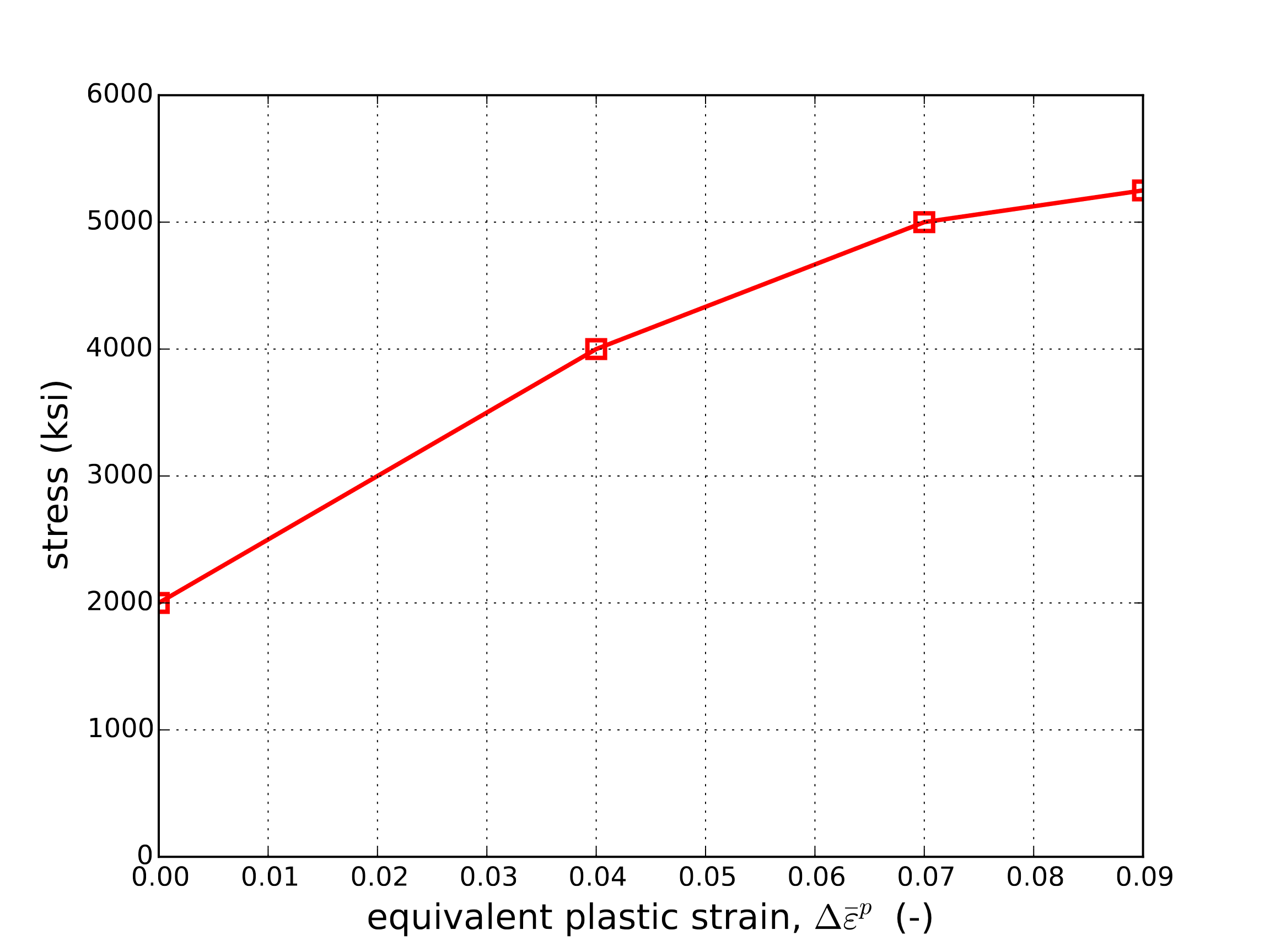
../../_images/mlep.png — Fig. 4.27 An example of a multilinear elastic-plastic stress-strain curve.

4.10.2. Implementation

The multilinear elastic-plastic model is implemented using a predictor-corrector algorithm. First, an elastic trial stress state is calculated. This is done in the unrotated configuration (see Section 4.1) by assuming that the rate of deformation is completely elastic

\[T^{tr}_{ij} = T^{n}_{ij} + \Delta t \left( \lambda\delta_{ij}d_{kk} + 2\mu d_{ij} \right).\]

The trial stress state is decomposed into a pressure and a deviatoric stress

\[p^{tr} = \frac{1}{3} T^{tr}_{kk} \;\;\; ; \;\;\; s^{tr}_{ij} = T^{tr}_{ij} - p^{tr}\delta_{ij}\]

The effective trial stress is calculated and used with the yield function~eqref{eq:EPyield},

\[f \left( s^{tr}_{ij},\bar{\varepsilon}^{p} \right) = \phi \left( s^{tr}_{ij} \right) - \bar{\sigma}\left( \bar{\varepsilon}^{p} \right).\]

If \(f \leq 0\) then the response is elastic and the stress update is finished. If \(f > 0\) then plastic deformation has occurred and a radial return algorithm is used to determine the extent of this behavior.

The model assumes associated flow such that the normal to the yield surface lies in the direction of the trial stress state. This leads to the following expression for the normal, \(N_{ij}\),

\[N_{ij} = \frac{s_{ij}^{tr}}{\|s_{ij}^{tr}\|}.\]

Using a backward Euler algorithm, the final deviatoric stress state may be written as

\[s^{n+1}_{ij} = s_{ij}^{tr} - \Delta \, t 2\mu d_{ij}^{\text{p}}\]

where the plastic strain increment, \(\Delta d_{ij}^{\text{p}}\), is

\[\Delta d_{ij}^{\text{p}} = \sqrt{\frac{3}{2}} \Delta\bar{\varepsilon}^{p} N_{ij}.\]

Thus, to determine the response of the material the increment of the effective plastic strain, \(\Delta\bar{\varepsilon}^p\), needs to be determined. This may be done by solving the linearized consistency equation over the load step that is written as,

\[3 \mu \Delta\bar{\varepsilon}^{p} + \bar{\sigma}\left( \bar{\varepsilon}_{n} + \Delta\bar{\varepsilon}^{p} \right) - \phi^{tr} + f_{n} = 0.\]

4.10.3. Verification

The multilinear elastic-plastic material model is verified for uniaxial stress and pure shear. The elastic properties used in these analyses are \(E = 70\) GPa and \(\nu = 0.25\). In order to appropriately verify this model, the hardening curve must have a functional form to appropriately determine an analytical solution. Here, the hardening law used for the model is a Voce law with the following form

\[\bar{\sigma}\left(\bar{\varepsilon}^{p}\right) = \sigma_{y} + A \left( 1 - \exp(-n \bar{\varepsilon}^{p})\right).\]

In the numerical analyses, this expression is discretized at a series of plastic strain values and used as input. For these calculations \(\sigma_{y} = 200\) MPa, \(A = 200\) MPa, and \(n = 20\).

4.10.3.1. Uniaxial Stress

The multilinear elastic-plastic model is tested in uniaxial tension. The test looks at the axial stress and the lateral strain and compares these values against analytical results for the same problem. In this verification problem only the normal strains/stresses are needed, and the shear terms are not exercised.

For the uniaxial stress problem, the only non-zero stress component is \(\sigma_{11}\). In the analysis that follows \(\sigma_{11} = \sigma\). There are three non-zero strain components, \(\varepsilon_{11}\), \(\varepsilon_{22}\), and \(\varepsilon_{33}\). In the analysis that follows \(\varepsilon_{11} = \varepsilon\) and \(\varepsilon_{22} = \varepsilon_{33}\). Furthermore, the axial elastic strain, \(\varepsilon_{11}^{\text{e}} = \sigma/E\) will be denoted by \(\varepsilon^{\text{e}}\).

The equivalent plastic strain, \(\bar{\varepsilon}^{\text{p}}\), for this model is equivalent to \(\varepsilon_{11}^{\text{p}}\), and is

\[\bar{\varepsilon}^{\text{p}} = \varepsilon - \frac{\bar{\sigma}\left(\bar{\varepsilon}^{\text{p}}\right)}{E}\]

This allows us, after yield, to parameterize the problem with the equivalent plastic strain.

For the lateral strains we need the lateral plastic strain. Incompressibility gives us

\[\bar{\varepsilon}^{\text{p}}_{22} = -\frac{1}{2}\bar{\varepsilon}^{\text{p}}\]

Combined with the lateral elastic strains we have the lateral strain as a function of the equivalent plastic strain

\[\varepsilon_{22} = -\nu\frac{\bar{\sigma}\left(\bar{\varepsilon}^{\text{p}}\right)}{E} - \frac{1}{2}\bar{\varepsilon}^{\text{p}}\]

The results are shown in Fig. 4.28 and Fig. 4.29 and show agreement between the model in Adagio and the analytical results.

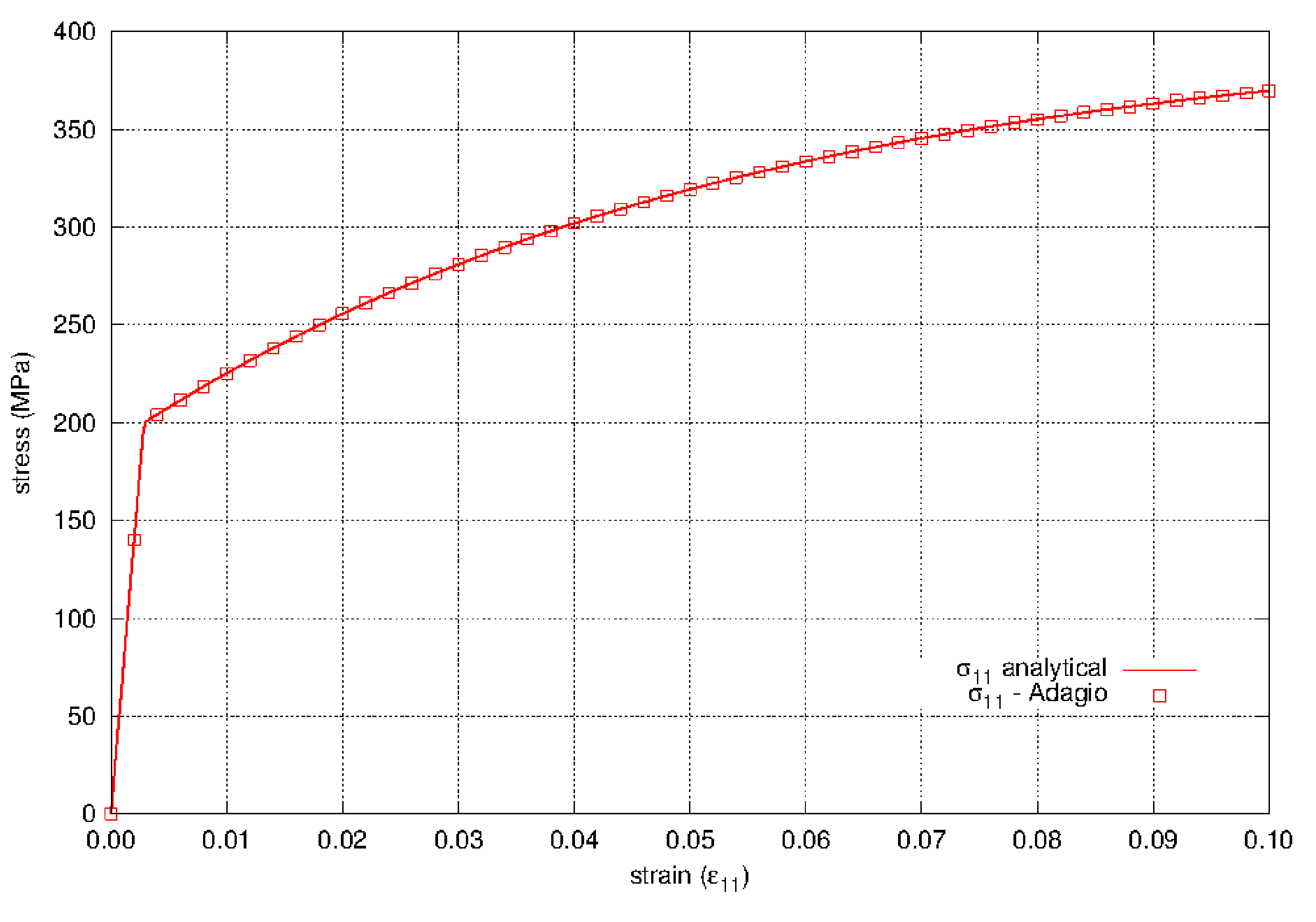
../../_images/multilinear_ep_uniaxial_stress2.png — Fig. 4.28 The axial stress as a function of axial strain for the multilinear elastic-plastic model with an analytical Voce law for the hardening model.

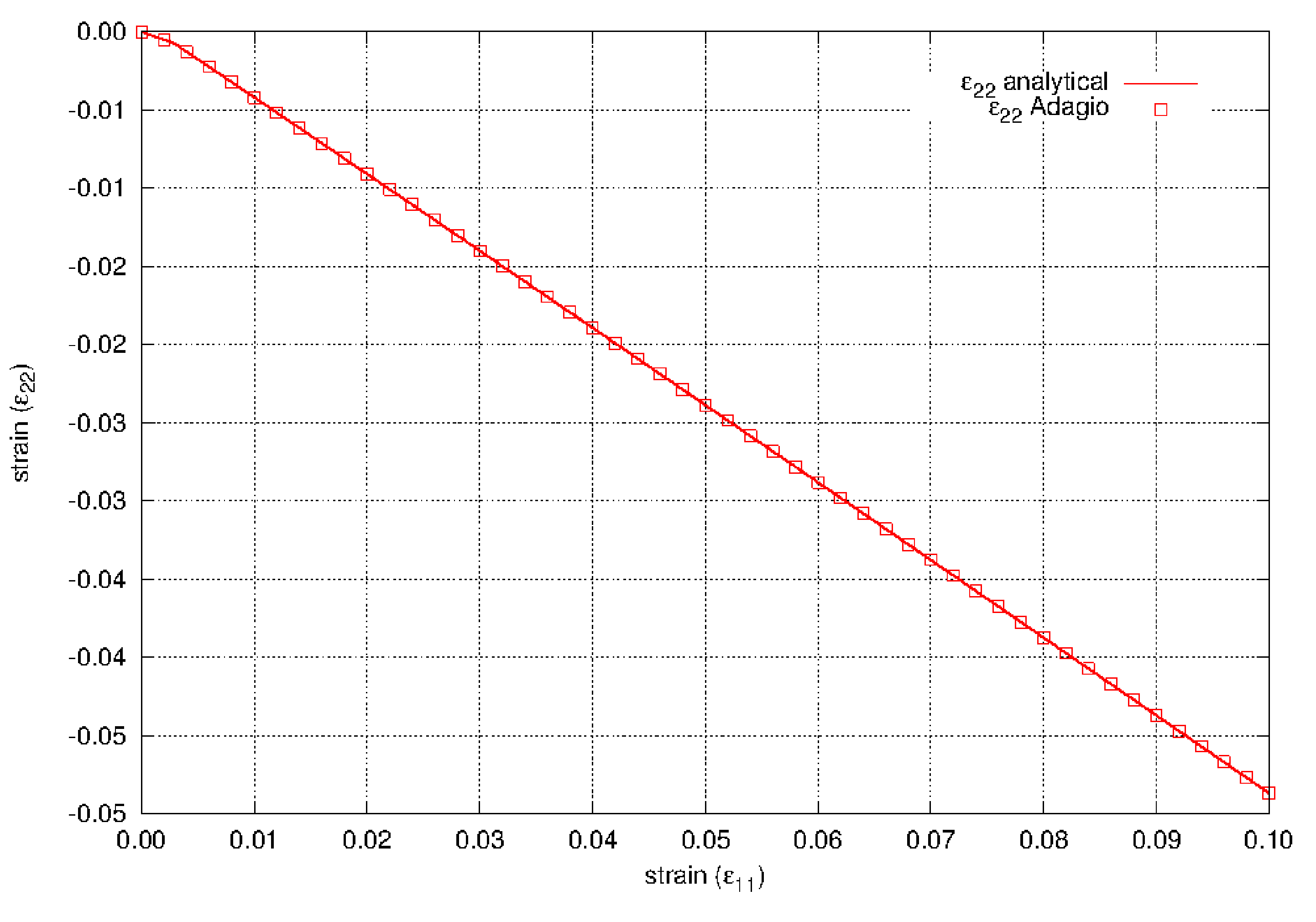
../../_images/multilinear_ep_uniaxial_stress1.png — Fig. 4.29 The lateral strain as a function of axial strain for the multilinear elastic-plastic model with an analytical Voce law for the hardening model.

4.10.3.2. Pure Shear

The multilinear elastic-plastic model is tested in pure shear. The test looks at the shear stress as a function of the shear strain and compares these values against analytical results for the same problem. For the pure shear problem, the only non-zero strain component is \(\varepsilon_{12}\) and the only non-zero stress component is \(\sigma_{12}\).

After yield, the shear stress as a function of the hardening curve is \(\sigma_{12} = \bar{\sigma}\left(\bar{\varepsilon}^{\text{p}}\right)/\sqrt{3}\). The elastic shear strain is \(\varepsilon_{12}^{\text{e}} = \sigma_{12}/2G\); the plastic shear strain is \(\varepsilon_{12}^{\text{p}} = \sqrt{3}\bar{\varepsilon}^{\text{p}}/2\). Using this, the shear stress and strain are given as functions of the equivalent plastic strain

\[\sigma_{12} = \frac{\bar{\sigma}\left(\bar{\varepsilon}^{\text{p}}\right)}{\sqrt{3}} \;\;\; ; \;\;\; \varepsilon_{12} = \frac{\sqrt{3}}{2} \bar{\varepsilon}^{\text{p}} + \frac{1}{\sqrt{3}}\frac{\bar{\sigma}\left(\bar{\varepsilon}^{\text{p}}\right)}{2G}\]

This allows us, after yield, to parameterize the problem with \(\bar{\varepsilon}^{\text{p}}\).

The results are shown in Fig. 4.30 and show agreement between the model in Adagio and the analytical results.

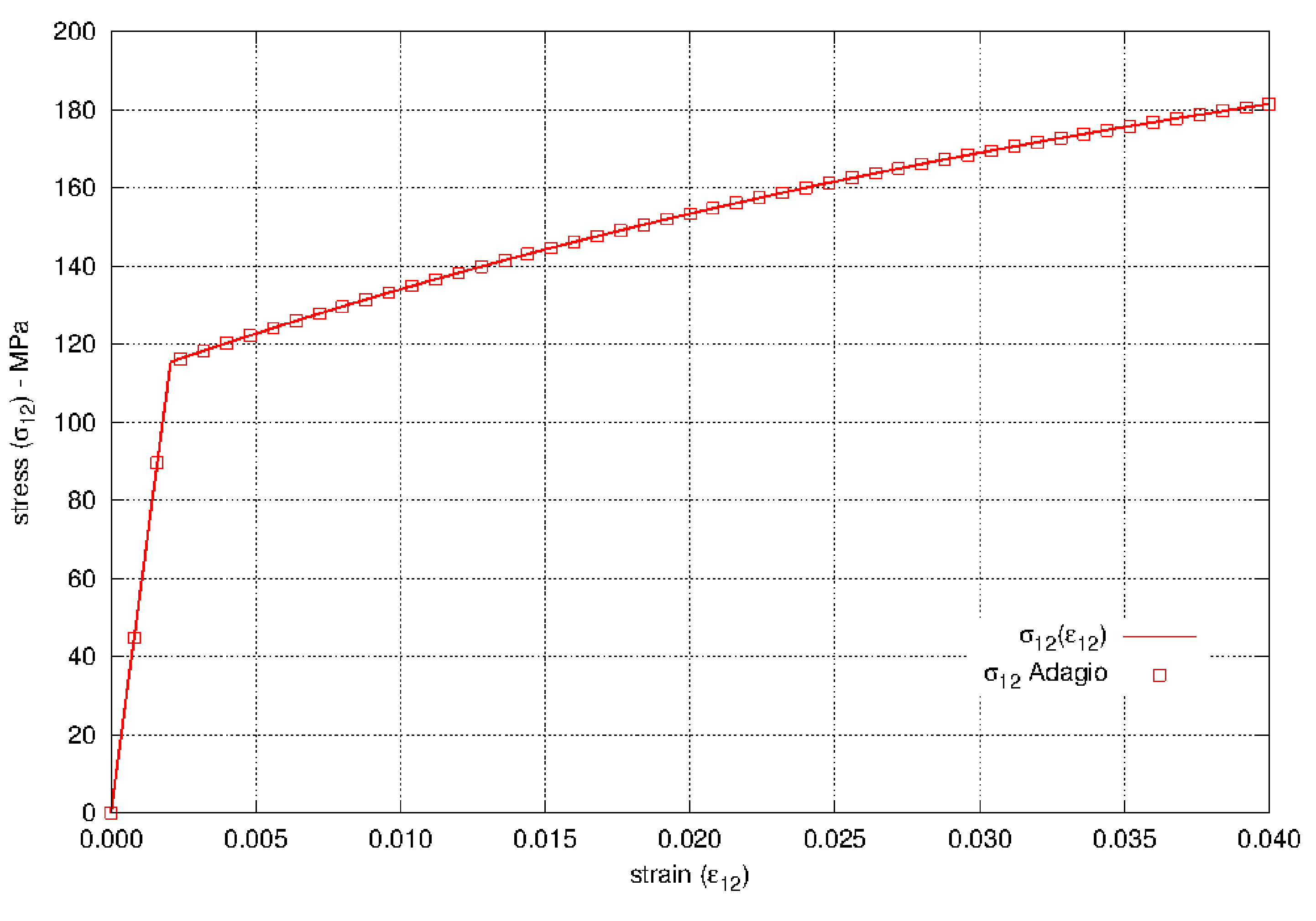
../../_images/multilinear_ep_pure_shear.png — Fig. 4.30 The shear stress as a function of shear strain for the multilinear elastic-plastic model with an analytical Voce law for the hardening model.

4.10.4. User Guide

 BEGIN PARAMETERS FOR MODEL MULTILINEAR_EP
  #
  # Elastic constants
  #
  YOUNGS MODULUS = <real>
  POISSONS RATIO = <real>
  SHEAR MODULUS  = <real>
  BULK MODULUS   = <real>
  LAMBDA         = <real>
  TWO MU         = <real>
  #
  # Hardening behavior
  #
  YIELD STRESS       = <real>
  BETA               = <real> (1.0)
  HARDENING FUNCTION = <string> hardening_function_name
  #
  # Functions
  #
  YOUNGS MODULUS FUNCTION = <string> ym_function_name
  POISSONS RATIO FUNCTION = <string> pr_function_name
  YIELD STRESS FUNCTION   = <string> yield_stress_function_name
END [PARAMETERS FOR MODEL MULTILINEAR_EP]

In the above command blocks:

The beta parameter defines if hardening is isotropic or kinematic.
YIELD STRESS defines the stress where plastic yielding first occurs.
The HARDENING FUNCTION command line references the name of a function defined in a FUNCTION command line in the SIERRA scope. The function describes the hardening behavior of the material as stress versus equivalent plastic strain. The x values of the function should be values of equivalent plastic strain while the y values of the function can be either the increment of stress over the yield stress or the actual stress at the corresponding equivalent plastic strain. Note the hardening function can have its first point defined at (0,0), or at (0, YIELD_STRESS). Either function definition behaves the same as only the slope of the hardening function between two strains is used by the model.
The YOUNGS MODULUS FUNCTION command line references the name of a function defined in a FUNCTION command line in the SIERRA scope that describes a scale factor on Young’s modulus as a function of temperature.
The POISSONS RATIO FUNCTION command line references the name of a function defined in a FUNCTION command line in the SIERRA scope that describes a scale factor on Poisson’s ratio as a function of temperature.
The YIELD STRESS FUNCTION command line references the name of a function defined in a FUNCTION command line in the SIERRA scope that describes a scale factor on the yield stress as a function of temperature.

Output variables available for this model are listed in Table 4.10 and Table 4.11.

Table 4.10 State Variables for MULTILINEAR EP Model
Name	Description
`EQPS`	equivalent plastic strain
`TENSILE_EQPS`	equivalent plastic strain only accumulated when the material is in tension (trace of stress tensor is positive)
`RADIUS`	radius of yield surface
`BACK_STRESS`	back stress (symmetric tensor)
`YOUNGS_MODULUS`	the current Young’s modulus as a function of temperature
`POISSONS_RATIO`	the current Poisson’s ratio as a function of temperature
`YIELD_STRESS`	the current yield stress as a function of temperature
`ITERATIONS`	radial return iterations
`YIELD_FLAG`	inside (0) or on (1) the yield surface

Table 4.11 State Variables for MULTILINEAR EP Model for Shells
Name	Description
`EQPS`	equivalent plastic strain
`TENSILE_EQPS`	equivalent plastic strain only accumulated when the material is in tension (trace of stress tensor is positive)
`RADIUS`	radius of yield surface
`BACK_STRESS`	back stress (symmetric tensor)
`YOUNGS_MODULUS`	the current Young’s modulus as a function of temperature
`POISSONS_RATIO`	the current Poisson’s ratio as a function of temperature
`YIELD_STRESS`	the current yield stress as a function of temperature
`ITERATIONS`	radial return iterations
`ERROR`	error in plane stress iterations
`PS_ITER`	plane stress iterations