4.6. Gent Model

4.6.1. Theory

The Gent model is a hyperelastic model of rubber elasticity developed from phenomenological continuum mechanics approaches. Specifically, the model is based on the concept of limiting chain extensibility and is an accurate approximation to the Arruda-Boyce model [[1]]. To determine the stress-strain response of the Gent model, a strain energy density of the form [[2]],

(4.15)\[W(B_{ij}) = \frac{1}{2}K\left[\frac{1}{2}\left( J^{2}-1 \right) - \ln J \right] + \frac{1}{2}\mu {J}_{m} \ln \left( 1- \frac{ \bar{B}_{kk} - 3}{{J}_{m}} \right),\]

is proposed with \(K\) and \(\mu\) the bulk and shear moduli, \(J\) the determinant of the deformation gradient and \(J_m\) an input parameter for limiting the value of \(\bar{B}_{kk}-3\). \(J_m\) is the parameter effectively accounting for limiting chain extensibility. The deformation measure is given by \(B_{ij}\), the components of the Left Cauchy Green tensor, where \(B_{ij} = F_{ik}F_{jk}\). \(\bar{B}_{kk}\) provides the isochoric part of the deformation and is given by

(4.16)\[\bar{B}_{ij} = \bar{F}_{ik}\bar{F}_{jk}~;~\bar{F}_{ij} = {J}^{-1/3}{F}_{ij}.\]

In the limit where \({J}_{m}\rightarrow\infty\) the Gent model reduces to the classical neo-Hookean model (see (4.8)). This can be seen by defining \(x\) to be \(\frac{1}{{J}_{m}}\), taking a Taylor series expansion of \(\ln \left(1-(\bar{B}_{kk}-3)x \right)\) about \(x=0\) and taking the limit as \(x\rightarrow0\).

The second Piola-Kirchoff stress, with components \(S_{ij}\), may be determined by taking a derivative of the strain energy density. A mapping of the second Piola-Kirchoff may be used to determined the Cauchy stress. These relations produce components of the Cauchy stress, \(\sigma_{ij}\), that are

(4.17)\[\sigma_{ij} = \frac{1}{2}K \left( J - \frac{1}{J} \right) \delta_{ij} + \frac{J^{-5/3}\mu{J}_{m}\left( B_{ij} - \frac{1}{3}B_{kk}\delta_{ij} \right)}{{J}_{m}-\bar{B}_{kk}+3},\]

where \(\delta_{ij}\) is the Kronecker delta.

The Gent model is a useful model for rubber elasticity as it is simple and provides similar predictions to comparatively complicated molecular models [[1], [3]]. It is also a practical model to use since analytic solutions to benchmark problems exist for this model.

4.6.2. Implementation

As a hyperelastic model, the current state of the material may be determined by the total deformation. To this end we use the polar decomposition of the deformation gradient,

(4.18)\[F_{ij} = V_{ik}R_{kj},\]

in which \(V_{ij}\) are the components of the left stretch tensor and \(R_{ij}\) is the corresponding rotation. Noting that,

\[B_{ij} = V_{ik}V_{kj},\]

and \(J=\det\left(V_{ij}\right)\), the Cauchy stress (via (4.17)) is found. The unrotated stress, \(T_{ij}\), which is needed for internal force calculations in Sierra/SM, is found using the transformation

\[T_{ij} = R_{ki}\sigma_{kl}R_{lj}.\]

4.6.3. Verification

It is possible to find closed form solutions for a number of loadings. Three problems are described here: uniaxial strain, simple shear, and hydrostatic compression. One set of material properties was used for all tests and they are given in Table 4.4. The elastic modulus and Poisson’s ratio are given in addition to the bulk modulus, shear modulus, and limiting chain extensibility parameter, \({J}_{m}\).

Table 4.4 The material properties for the Gent model used for uniaxial strain, simple shear, and hydrostatic compression tests.

\(K\)	0.325 MPa	\(\mu\)	0.15 MPa	\(J_m\)	13.125
\(E\)	0.39 MPa	\(\nu\)	0.33

4.6.3.1. Uniaxial Strain

First, utilizing a displacement condition corresponding to uniaxial strain results in a deformation gradient of the form,

\[F_{ij}=\lambda\delta_{1i}\delta_{1j} + \delta_{2i}\delta_{2j}+\delta_{3i}\delta_{3j}.\]

By evaluating relation (4.17) with this deformation field, we produce stresses that may be written as,

\[\begin{split}\sigma_{11} & = \frac{1}{2}K\left(\lambda-\frac{1}{\lambda}\right)-\frac{2}{3}\frac{J_m\mu\left(\lambda^2-1\right)}{\lambda^3-\left(J_m+3\right)\lambda^{5/3}+2\lambda} \nonumber \\ \\ \sigma_{22} = \sigma_{33} & = \frac{1}{2}K\left(\lambda-\frac{1}{\lambda}\right)+\frac{1}{3}\frac{J_m\mu\left(\lambda^2-1\right)}{\lambda^3-\left(J_m+3\right)\lambda^{5/3}+2\lambda}, \nonumber\end{split}\]

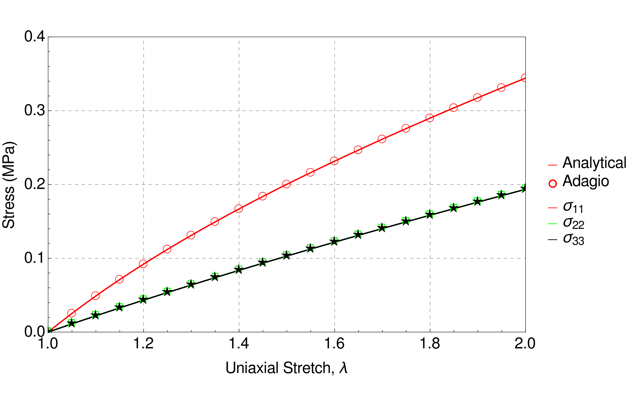
Fig. 4.13 Analytical and numerical results for the uniaxial stretch case.

with the shear stress components equal to zero. Both the corresponding analytical and numerical solutions are presented in Fig. 4.13.

4.6.3.2. Simple Shear

For the simple shear case, a deformation gradient of the form,

\[F_{ij}=\delta_{ij}+\gamma\delta_{1i}\delta_{2j},\]

is assumed. Noting this is a volume preserving deformation (\(J=1\)) and again evaluating (4.17) produces stresses that may be written as,

\[\begin{split}\sigma_{11} & = \frac{2}{3}\frac{J_m\mu\gamma^2}{J_m-\gamma^2} \nonumber \\ \nonumber \\ \sigma_{22}=\sigma_{33} & = -\frac{1}{3}\frac{J_m\mu\gamma^2}{J_m-\gamma^2} \\ \nonumber \\ \sigma_{12} & = \frac{J_m\mu\gamma}{J_m-\gamma^2} \nonumber\end{split}\]

Both the corresponding analytical and numerical solutions are presented in Fig. 4.14.

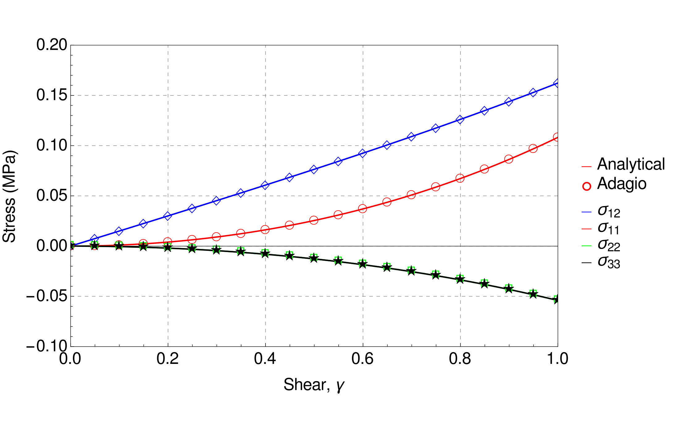
Fig. 4.14 Analytical and numerical results for the simple shear case.

4.6.3.3. Hydrostatic Compression

The volumetric deformation capabilities of the model are also investigated through displacement controlled hydrostatic compression. Specifically, hydrostatic compression results in a deformation gradient of the form,

\[F_{ij}=\lambda\delta_{ij},\]

where 0 \(<\) \(\lambda\) \(\leq\) 1. As there is no deviatoric deformation, evaluation of (4.17) produces stresses that may be written as,

\[\sigma_{11}=\sigma_{22}=\sigma_{33} = \frac{1}{2}K\left(\lambda^3-\frac{1}{\lambda^3}\right),\]

with the shear stress components equal to zero. Both the corresponding analytical and numerical solutions are presented in Fig. 4.15.

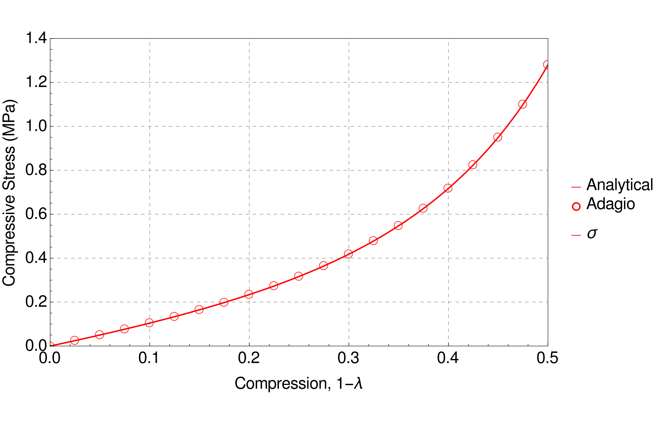
Fig. 4.15 Stress determined analytically and numerically for the Gent model during displacement controlled hydrostatic compression.

4.6.4. User Guide

BEGIN PARAMETERS FOR MODEL GENT
  #
  # Elastic constants
  #
  YOUNGS MODULUS = <real>
  POISSONS RATIO = <real>
  SHEAR MODULUS  = <real>
  BULK MODULUS   = <real>
  LAMBDA         = <real>
  TWO MU         = <real>
  #
  Jm Parameter  = <real>
END [PARAMETERS FOR MODEL GENT]

There are no output variables available for the Gent model.

---

[1] (1,2)

Ellen M Arruda and Mary C Boyce. A three-dimensional constitutive model for the large stretch behavior of rubber elastic materials. Journal of the Mechanics and Physics of Solids, 41(2):389–412, 1993. doi:10.1016/0022-5096(93)90013-6.

[2]

A.N. Gent. A new constitutive relation for rubber. Rubber Chemistry and Technology, 69(1):59–61, 1996.

[3]

Michael R. Buche and Meredith N. Silberstein. Statistical mechanical constitutive theory of polymer networks: The inextricable links between distribution, behavior, and ensemble. Phys. Rev. E, 102:012501, Jul 2020. doi:10.1103/PhysRevE.102.012501.