4.33. Linear Thermoviscoelastic Model

4.33.1. Theory

The linear thermoviscoelastic model (LTVE for short) is, as the name implies, a phenomenological thermoviscoelasticity model. This formulation seeks to provide a similar, albeit simpler and more adaptable, form versus the complexity of models like the UNIVERSAL_POLYMER_MODEL based on the potential energy clock (PEC) or simplified potential energy clock (SPEC). Further, to aid in the adaptability of the new model a modular shift factor capability is added.

For a general perspective, the LTVE model is a continuum thermodynamics based, hereditary integral viscoelastic formulation. The basic theory is quite similar to that found in Christensen [[1]] with some extra observations and assumptions found in the PEC/SPEC formalisms [[2], [3]]. To begin, external state variables of the total strain, \(\varepsilon_{ij}\), absolute temperature, \(\theta\), and time, \(t\), are used. No additional internal state variables are needed. A Helmholtz free energy, \(\psi\), is introduced such that

\[\psi\left(\varepsilon_{ij},\theta,t\right)=\psi^{\infty}\left(\varepsilon_{ij},\theta\right)+\psi^{\text{neq}}\left(\varepsilon_{ij},\theta,t\right),\]

with \(\psi^{\infty}\) and \(\psi^{\text{neq}}\) being the equilibrium energy describing the free-energy of the equilibrium phase and non-equilibrium energy associated with the additional energy of the glassy phase yet to be relaxed, respectively. The former term may be given as,

\[\psi^{\infty}=\frac{1}{2\rho}\left(\varepsilon_{ij}-\bar{\alpha}^{\infty}\left(\theta-\theta_0\right)\delta_{ij}\right)\bar{\mathbb{C}}_{ijkl}^{\infty} \left(\varepsilon_{kl}-\bar{\alpha}^{\infty}\left(\theta-\theta_0\right)\delta_{kl}\right)+\psi_{\theta}^{\infty}\left(T\right),\]

where \(\rho\), \(\bar{\alpha}^{\infty}\), \(\theta_0\), and \(\bar{\mathbb{C}}_{ijkl}^{\infty}\) are, respectively, the material density, current linear coefficient of thermal expansion, reference temperature, and current equilibrium stiffness tensor. A purely thermal contribution, \(\psi_{\theta}^{\infty}\), is also included in the free energy but does not contribute to the mechanical response and as such is not explicitly defined at this point. In the previous and following relations, an overbar, \(~\bar{\cdot}~\), denotes a temperature dependent quantity such that \(\bar{x}=xf^x\left(\theta\right)\) with \(x\) being the reference constant value and \(f^x\left(\theta\right)\) being a temperature dependent multiplier that should be order one. To capture the non-equilibrium contribution, the corresponding free-enery term is written,

\[\begin{split}\psi^{\text{neq}} & = \frac{\Delta \bar{K}}{2\rho}\int_0^t\int_0^tf_v\left(t^*-s^*,t^*-u^*\right)\frac{\partial\varepsilon_{kk}}{\partial s}\frac{\partial\varepsilon_{mm}}{\partial u}dsdu \\ & +\frac{\Delta\bar{\mu}}{\rho}\int_0^t\int_0^tf_s\left(t^*-s^*,t^*-u^*\right)\frac{\partial\varepsilon_{ij}^{\prime}}{\partial s}\frac{\partial\varepsilon_{ij}^{\prime}}{\partial u}dsdu \\ & -\frac{3\Delta\left(\bar{\alpha} \bar{K}\right)}{\rho}\int_0^t\int_0^t f_v\left(t^*-s^*,t^*-u^*\right)\frac{\partial \theta}{\partial s}\frac{\partial\varepsilon_{kk}}{\partial u}dsdu \\ & +\psi_{\theta}^{\text{neq}}\left(\theta,t\right),\end{split}\]

in which \(\Delta\) denotes the difference in a glassy and equilibirium property (\(\Delta \bar{x} = \bar{x}^g-\bar{x}^{\infty}\)), \(K\) and \(\mu\) are bulk and shear moduli, and \(\psi_{\theta}^{\text{neq}}\) is a purely thermal term that does not currently impact the mechanical theory. The prior relation also included two terms related to viscoelastic spectra – \(f_v\) and \(f_s\) – with the former being related to volumetric terms and the later shear. Further, a \(*\) indicates a quantity taken in the material time that is shifted from the laboratory time. These two scales are related via a shift factor, \(a\), such that,

\[t^* = \int_0^t\frac{ds}{a\left(s\right)}.\]

While different shift factors are allowed via the modular framework, it should be noted they are restricted to those that are a function of temperature (and potentially time) alone. Non-linear shift factors involving things like deformation measures are not permitted.

Following conventional continuum thermodynamic arguments, the Cauchy stress may be determined to be,

(4.167)\[\begin{split}\sigma_{ij} & = \bar{K}^{\infty}\left(\varepsilon_{kk}-3\bar{\alpha}^{\infty}\left(\theta-\theta_0\right)\right)\delta_{ij}+2\bar{\mu}^{\infty}\varepsilon_{ij}^{\prime} \\ & +\Delta \bar{K} J^1\delta_{ij}-3\Delta\left(\bar{\alpha} \bar{K}\right)J^3\delta_{ij}+2\Delta\bar{\mu} J_{ij}^2,\end{split}\]

where \(J^1,~J^2_{ij},\) and \(J^3\) are representations of the hereditary integrals given by,

\[\begin{split}J^1 & = \int_0^t f_v\left(t^*-s^*\right)\frac{\partial\varepsilon_{kk}}{\partial s} ds, \\ J^2_{ij} & = \int_0^t f_s\left(t^*-s^*\right)\frac{\partial \varepsilon_{ij}^{\prime}}{\partial s} ds, \\ J^3 & = \int_0^t f_v\left(t^*-s^*\right)\frac{\partial \theta}{\partial s} ds.\end{split}\]

4.33.1.1. Modular Shift Factor

To provide enhanced flexibility to the user, the shift factor was implemented in a modular fashion such that four different functional forms can be used. The first two are well-established analytical forms – Williams-Landel-Ferry (WLF) [[4]] and Arrhenius. These forms are given by,

\[\begin{split}\text{log}_{10}a^{\text{WLF}} & = \frac{-C_1\left(\theta-\theta_{\text{ref}}\right)}{C_2+\left(\theta-\theta_{\text{ref}}\right)}, \\ \text{log}_{10}a^{\text{Arr}} & = \frac{E_a}{R}\left(\text{log}_{10}\text{e}\right)\left(\frac{1}{\theta}-\frac{1}{\theta_{\text{ref}}}\right),\end{split}\]

with \(C_1,~C_2,\) and \(\theta_{\text{ref}}\) being fit parameters for the WLF expression and \(E_a\) and \(R\) are the activation energy and gas constant for the Arrhenius energy, respectively. To enable direct utilization of experimental determination of the shift factor, the third option is a user-defined shift factor that is explicitly a function of temperature such that,

\[a = a^{\text{ud}}\left(\theta\right),\]

in which \(a^{\text{ud}}\) is any user-defined Sierra scope function. Additionally, to be clear, the Sierra function should define the actual shift factor and not its logarithm.

Finally, the fourth option for the modular shift factor is defined to introduce history dependence in the cooling rate. This shift factor is referred to as WLF_LAG and is the WLF term with an extra thermal history dependence integral and is equivalent to the SPEC shift factor with \(C_3=C_4=0\) and is written,

\[\text{log}_{10}a^{\text{WLF\_LAG}} = \frac{ -C_1\left( \theta-\theta_\text{ref}-\int_0^{tf_v}\left(t^*-s^*\right)\frac{\partial\theta}{\partial s}ds \right) }{ C_2+\left( \theta-\theta_{\text{ref}}-\int_0^{tf_v}\left(t^*-s^*\right)\frac{\partial\theta}{\partial s}ds \right) }.\]

For more details please see [[5]]

4.33.2. Implementation

To implement the LTVE model, a fully implicit, backward Euler hypoelastic approach is utilized to integrate the model from a time \(t_n\) to a new time \(t_{n+1}\) with \(\Delta t = t_{n+1}-t_{n}\). The material state at time \(t_n\) is taken to be completely known. Loading is prescribed via a total strain rate, \(\dot{\varepsilon}^{n+1}_{ij}\), such that \(\varepsilon_{ij}^{n+1}=\varepsilon_{ij}^n+\Delta t \dot{\varepsilon}_{ij}^{n+1}\), and prescribed temperature history such that \(\theta^{n+1}=\theta\left(t_{n+1}\right)\) is known. Objectivity is satisfied through the standard approaches described in Section 4.1.

In such an implicit form, the updated stress is written

\[\sigma_{ij}^{n+1}=\sigma_{ij}^n+\Delta t \dot{\sigma}_{ij}^{n+1}.\]

The rate of change of the stress, \(\dot{\sigma}_{ij}\), may be found by differentiating (4.167) and written as,

\[\begin{split}\dot{\sigma}_{ij} & = \bar{K}^{\infty}\dot{\varepsilon}_{kk}\delta_{ij}+2\bar{\mu}^{\infty}\dot{\varepsilon}_{ij}^{\prime} +\Delta\bar{K}\dot{J}^1\delta_{ij}-3\Delta\left(\bar{\alpha}\bar{K}\right)\dot{J}^3\delta_{ij}-3\bar{K}^{\infty} \bar{\alpha}^{\infty}\dot{\theta}\delta_{ij}+2\Delta\bar{\mu}\dot{J}_{ij}^2 \nonumber \\ & -3\dot{\theta}\delta_{ij}\left(\left(\frac{\partial\bar{K}^{\infty}}{\partial\theta}\bar{\alpha}^{\infty}+ \bar{K}^{\infty}\frac{\partial\bar{\alpha}^{\infty}}{\partial\theta}\right)\left(\theta-\theta_0\right)+ \frac{\partial\left(\Delta\bar{\alpha}\bar{K}\right)}{\partial\theta}J^3 -\frac{1}{3}\frac{\partial\bar{K}^{\infty}}{\partial\theta}\varepsilon_{kk} -\frac{1}{3}\frac{\partial\left(\Delta\bar{K}\right)}{\partial\theta}J^1\right) \nonumber \\ & +2\dot{\theta}\left(\frac{\partial\bar{\mu}^{\infty}}{\partial\theta}\varepsilon_{ij}^{\prime} +\frac{\partial\left(\Delta\bar{\mu}\right)}{\partial\theta}J_{ij}^2\right)\end{split}\]

In the preceeding relation, the latter two lines pertain purely to changes in temperature dependent thermoelastic properties. With the strain rate, current strain, and current temperature prescribed as inputs, expressions for the temperature rate, hereditary integral rates, and current values of the hereditary integral are needed. The first may be simply numerically approximated via,

\[\dot{\theta}^{n+1}\approx\frac{\theta^{n+1}-\theta^n}{\Delta t}.\]

The actual expression for the hereditary integral has not been defined to this point. The choice and selection of these functions has long been studied as the ability to accurately and efficiently numerically integrate them is essential for making the models tractable. This problem has been tackled previously through the judicious use of exponential functions. To this end, the forms proposed by Caruthers et al. [[2]] are used and are written,

\[f_{v,s}\left(t^*-s^*,t^*-u^*\right)=\sum_{k=1}^{n_{v,s}}w_k^{v,s}\exp\left(-\frac{t^*-s^*}{\tau_k^{v,s}}\right) \exp\left(-\frac{t^*-u^*}{\tau_k^{v,s}}\right),\]

where \(v,s\) indicate either the volumetric or shear spectra and \(w_k\) and \(\tau_k\) are the corresponding charastic weight and time, respecitvely, of the \(k-\text{th}\) prony term. The number of prony terms is denoted \(n_{v,s}\).

The first herediatry integral term may be written,

(4.168)\[J^1 = \sum_{n=1}^{n_v}w_k^vJ^{1\left(k\right)},~\qquad\qquad~J^{1\left(k\right)}=\int_0^t\exp\left(-\frac{t^*-s^*}{\tau_k^v} \right)\frac{\partial\varepsilon_{mm}}{\partial s}ds.\]

For simplicity in what follows, only the integration of \(J^1\) is presented although similar approaches may be followed for \(J_{ij}^2\) and \(J^3\). Differentiating the two expressions in (4.168) yields,

(4.169)\[\dot{J}^1 = \sum_{k=1}^{n_v}w_k^v\dot{J}^{1\left(k\right)},\]

(4.170)\[\dot{J}^{1\left(k\right)} = \dot{\varepsilon}_{mm}-\frac{1}{\tau_k^v}\frac{dt^*}{dt}\int_0^t\exp \left(-\frac{t^*-s^*}{\tau_k^v}\right)\frac{\partial\varepsilon_{mm}}{\partial s}ds = \dot{\varepsilon}_{mm} - \frac{1}{a\tau_k^v}J^{1\left(k\right)}.\]

With these expressions, it is clear that first step in updating \(J_1\) is updating the various characteristic components. Each of these may be integrated implicitly via,

\[J_{n+1}^{1\left(k\right)} = J_n^{1\left(k\right)}+\Delta t\dot{J}_{n+1}^{1\left(k\right)}.\]

Using (4.170), the updated characteristic component of the hereditary integral is written,

\[J_{n+1}^{1\left(k\right)} = \frac{a^{n+1}\tau_k^v}{a^{n+1}\tau_k^v+\Delta t}\left(J_n^{1\left(k\right)} + \Delta t\dot{\varepsilon}_{mm}^{n+1}\right).\]

With all of the components identified, the updated stress becomes,

\[\begin{split}\sigma_{ij}^{n+1} & = \sigma_{ij}^n+\hat{K}d\varepsilon_{kk}\delta_{ij}+2\hat{\mu}d\varepsilon_{ij}^{\prime} - 3\left(\hat{K\alpha}\right)d\theta\delta_{ij} \nonumber \\ & -\Delta\bar{K}\sum_{k=1}^{n_v}\frac{w_k^v\Delta t}{a\tau_k^v+\Delta t}\left(J_n^{1\left(k\right)}+ d\varepsilon_{mm}\right)\delta_{ij}-2\Delta\bar{\mu}\sum_{k=1}^{n_s}\frac{w_k^s\Delta t}{a\tau_k^s+\Delta t} \left(J_{ij}^{2\left(k\right)\left(n\right)}+d\varepsilon_{ij}^{\prime}\right) \nonumber \\ & + 3\Delta\left(\bar{\alpha}\bar{K}\right)\sum_{k=1}^{n_v}\frac{w_k^v\Delta t}{a\tau_k^v+\Delta t} \left(J_n^{3\left(k\right)}+d\theta\right) \nonumber \\ & -3d\theta\delta_{ij}\left(\left(\theta-\theta_0\right)\left(\frac{\partial\bar{K}^{\infty}}{\partial\theta}\bar{\alpha}^{\infty} +\bar{K}^{\infty}\frac{\partial\bar{\alpha}}{\partial\theta}\right)+\frac{\partial\left(\Delta\bar{\alpha}\bar{K}\right)}{\partial\theta} \sum_{k=1}^{n_v}w_k^v\left(\frac{a\tau_k^v}{a\tau_k^v+\Delta t}\right)\left(d\theta+J_n^{3\left(k\right)}\right)\right) \nonumber \\ & +d\theta\left(\frac{\partial\bar{K}^{\infty}}{\partial\theta}\varepsilon_{kk}^{n+1}\delta_{ij}+2\frac{\partial\bar{\mu}^{\infty}}{\partial\theta} \varepsilon_{ij}^{\prime\left(n+1\right)}+\frac{\partial\left(\Delta\bar{K}\right)}{\partial\theta}\delta_{ij} \sum_{k=1}^{n_v}w_k^v\left(\frac{a\tau_k^v}{a\tau_k^v+\Delta t}\right)\left(J_n^{1\left(k\right)}+d\varepsilon_{mm}\right)\right. \nonumber \\ & \left.+2\frac{\partial\Delta\bar{\mu}}{\partial\theta}\sum_{k=1}^{n_s}w_k^s\left(\frac{a\tau_k^s}{a\tau_k^s+\Delta t}\right) \left(J_{ij}^{2\left(k\right)\left(n\right)}+d\varepsilon_{ij}^{\prime}\right) \right),\end{split}\]

with \(d\theta = \theta^{n+1}-\theta^{n}\), \(d\varepsilon_{ij}=\dot{\varepsilon}_{ij}\Delta t\), and

\[\begin{split}\hat{K} := & \bar{K}^{\infty} + \Delta\bar{K}\sum_{k=1}^{n_v}w_k^v, \\ \hat{\mu} := & \bar{\mu}^{\infty}+\Delta\bar{\mu}\sum_{k=1}^{n_s}w_k^s, \\ \left(\hat{\alpha K}\right) := & \bar{K}^{\infty}\bar{\alpha}^{\infty} + \Delta\left(\bar{\alpha}\bar{K}\right)\sum_{k=1}^{n_v}w_k^v.\end{split}\]

4.33.3. Verification

To verify the LTVE model, a series of verification exercises have been pursued. For these activities the viscoelastic parameterization provided by Kuether [[6]] are used in which model parameters are given in Table 4.53 and the viscoelastic spectra in Table 4.54. Given the rate-dependent nature of the viscoelastic models, analytical solutions are generally not available. As such, semi-analytic approaches are generally pursued through a variety of loadings.

Table 4.53 Model parameters for the linear thermoviscoelastic model from Kuether.

\(K^{\infty}\)	3.2 GPa	\(K^g\)	4.9 GPa
\(G^{\infty}\)	4.5 MPa	\(G^g\)	752 MPa
\(C_1\)	16.5 (-)	\(C_2\)	54.3 (\({}^{o}\)C)
\(T_{\text{ref}}\)	75 (\({}^{o}\)C)	\(E_a/R\)	3928 (\({}^{o}\)C)

Table 4.54 Viscoelastic strectra for the linear thermoviscoelastic model from Kuether.

term	\(\tau_k^v\) (s)	\(w_k^v\) (-)	\(\tau_k^s\) (s)	\(w_k^s\) (-)
1	\(1.0\times 10^{-10}\)	\(1.06\times 10^{-2}\)	\(1.0\times 10^{-10}\)	\(4.96\times 10^{-3}\)
2	\(1.0\times 10^{-9}\)	\(1.14\times 10^{-2}\)	\(1.0\times 10^{-9}\)	\(6.85\times 10^{-3}\)
3	\(1.0\times 10^{-8}\)	\(1.64\times 10^{-2}\)	\(1.0\times 10^{-8}\)	\(1.14\times 10^{-2}\)
4	\(1.0\times 10^{-7}\)	\(2.27\times 10^{-2}\)	\(1.0\times 10^{-7}\)	\(1.97\times 10^{-2}\)
5	\(1.0\times 10^{-6}\)	\(2.63\times 10^{-2}\)	\(1.0\times 10^{-6}\)	\(2.64\times 10^{-2}\)
6	\(3.16\times 10^{-6}\)	\(8.85\times 10^{-3}\)	\(3.16\times 10^{-6}\)	\(1.13\times 10^{-2}\)
7	\(1.0\times 10^{-5}\)	\(2.52\times 10^{-2}\)	\(1.0\times 10^{-5}\)	\(2.98\times 10^{-2}\)
8	\(3.16\times 10^{-5}\)	\(1.94\times 10^{-2}\)	\(3.16\times 10^{-5}\)	\(2.75\times 10^{-2}\)
9	\(1.0\times 10^{-4}\)	\(2.80\times 10^{-2}\)	\(1.0\times 10^{-4}\)	\(4.02\times 10^{-2}\)
10	\(3.16\times 10^{-4}\)	\(2.83\times 10^{-2}\)	\(3.16\times 10^{-4}\)	\(4.58\times 10^{-2}\)
11	\(1.0\times 10^{-3}\)	\(3.41\times 10^{-2}\)	\(1.0\times 10^{-3}\)	\(5.76\times 10^{-2}\)
12	\(3.16\times 10^{-3}\)	\(3.70\times 10^{-2}\)	\(3.16\times 10^{-3}\)	\(6.74\times 10^{-2}\)
13	\(1.0\times 10^{-2}\)	\(4.19\times 10^{-2}\)	\(1.0\times 10^{-2}\)	\(7.90\times 10^{-2}\)
14	\(3.16\times 10^{-2}\)	\(4.58\times 10^{-2}\)	\(3.16\times 10^{-2}\)	\(8.85\times 10^{-2}\)
15	\(1.0\times 10^{-1}\)	\(5.02\times 10^{-2}\)	\(1.0\times 10^{-1}\)	\(9.56\times 10^{-2}\)
16	\(3.16\times 10^{-1}\)	\(5.39\times 10^{-2}\)	\(3.16\times 10^{-1}\)	\(9.72\times 10^{-2}\)
17	\(1.0\times 10^{0}\)	\(5.71\times 10^{-2}\)	\(1.0\times 10^{0}\)	\(9.17\times 10^{-2}\)
18	\(3.16\times 10^{0}\)	\(5.93\times 10^{-2}\)	\(3.16\times 10^{0}\)	\(7.79\times 10^{-2}\)
19	\(1.0\times 10^{1}\)	\(6.03\times 10^{-2}\)	\(1.0\times 10^{1}\)	\(5.75\times 10^{-2}\)
20	\(3.16\times 10^{1}\)	\(5.97\times 10^{-2}\)	\(3.16\times 10^{1}\)	\(3.49\times 10^{-2}\)
21	\(1.0\times 10^{2}\)	\(5.72\times 10^{-2}\)	\(1.0\times 10^{2}\)	\(1.63\times 10^{-2}\)
22	\(3.16\times 10^{2}\)	\(5.30\times 10^{-2}\)	\(3.16\times 10^{2}\)	\(5.26\times 10^{-3}\)
23	\(1.0\times 10^{3}\)	\(4.66\times 10^{-2}\)	\(1.0\times 10^{3}\)	\(1.05\times 10^{-3}\)
24	\(3.16\times 10^{3}\)	\(3.95\times 10^{-2}\)	\(3.16\times 10^{3}\)	\(8.72\times 10^{-5}\)
25	\(1.0\times 10^{4}\)	\(3.03\times 10^{-2}\)	\(1.0\times 10^{4}\)	\(1.29\times 10^{-5}\)
26	\(3.16\times 10^{4}\)	\(2.34\times 10^{-2}\)	\(1.0\times 10^{5}\)	\(2.67\times 10^{-6}\)
27	\(1.0\times 10^{5}\)	\(1.34\times 10^{-2}\)	\(1.0\times 10^{6}\)	\(4.17\times 10^{-7}\)
28	\(3.16\times 10^{5}\)	\(1.12\times 10^{-2}\)
29	\(1.0\times 10^{6}\)	\(1.56\times 10^{-2}\)
30	\(3.16\times 10^{6}\)	\(4.84\times 10^{-3}\)

4.33.3.1. Balanced Biaxial Creep

For the first test of the LTVE model, the creep response under a balanced biaxial load is investigated. For this case, the stress state reduces to,

\[\begin{split}\sigma_{ij}\left(t\right) = \left[\begin{array}{ccc} \sigma\left(t\right) & 0 & 0 \\ 0 & -\sigma\left(t\right) & 0 \\ 0 & 0 & 0\end{array}\right].\end{split}\]

Under a constant temperature, \(\theta\left(t\right)=\theta\left(t_0\right)\), the stress state remains deviatoric through loading such that \(\sigma^{\prime}_{ij}\left(t\right)=\sigma_{ij}\left(t\right)\) thereby reducing the stress tensor to

(4.171)\[\sigma_{ij}=2\mu^{\infty}\varepsilon_{ij}+2\Delta\mu J_{ij}^2.\]

With these prescribed, only the strain remains unknown to be determined. Given the assumed stress state, the strains may also be related via \(\varepsilon_{yy}=-\varepsilon_{xx}\) reducing the problem to a single unknown. Following the implicit integration approaches discussed in the numerical implementation section, a semi-analytic expression for the strain is written,

(4.172)\[\varepsilon_{xx}^{n+1} = \frac{\sigma_{xx}^{n+1}-2\Delta\mu\sum_{i=1}^{n_s}w_k^s\frac{a^{n+1}\tau_k^s}{a^{n+1}\tau_k^s+\Delta t} \left(J_{xx}^{2\left(k\right)\left(n+1\right)}-\varepsilon_{xx}^n\right)}{2\left(\mu^{\infty}+\Delta\mu\sum_{i=1}^{n_s}w_k^s\frac{a^{n+1}\tau_k^s}{a^{n+1}\tau_k^s+\Delta t}\right)}\]

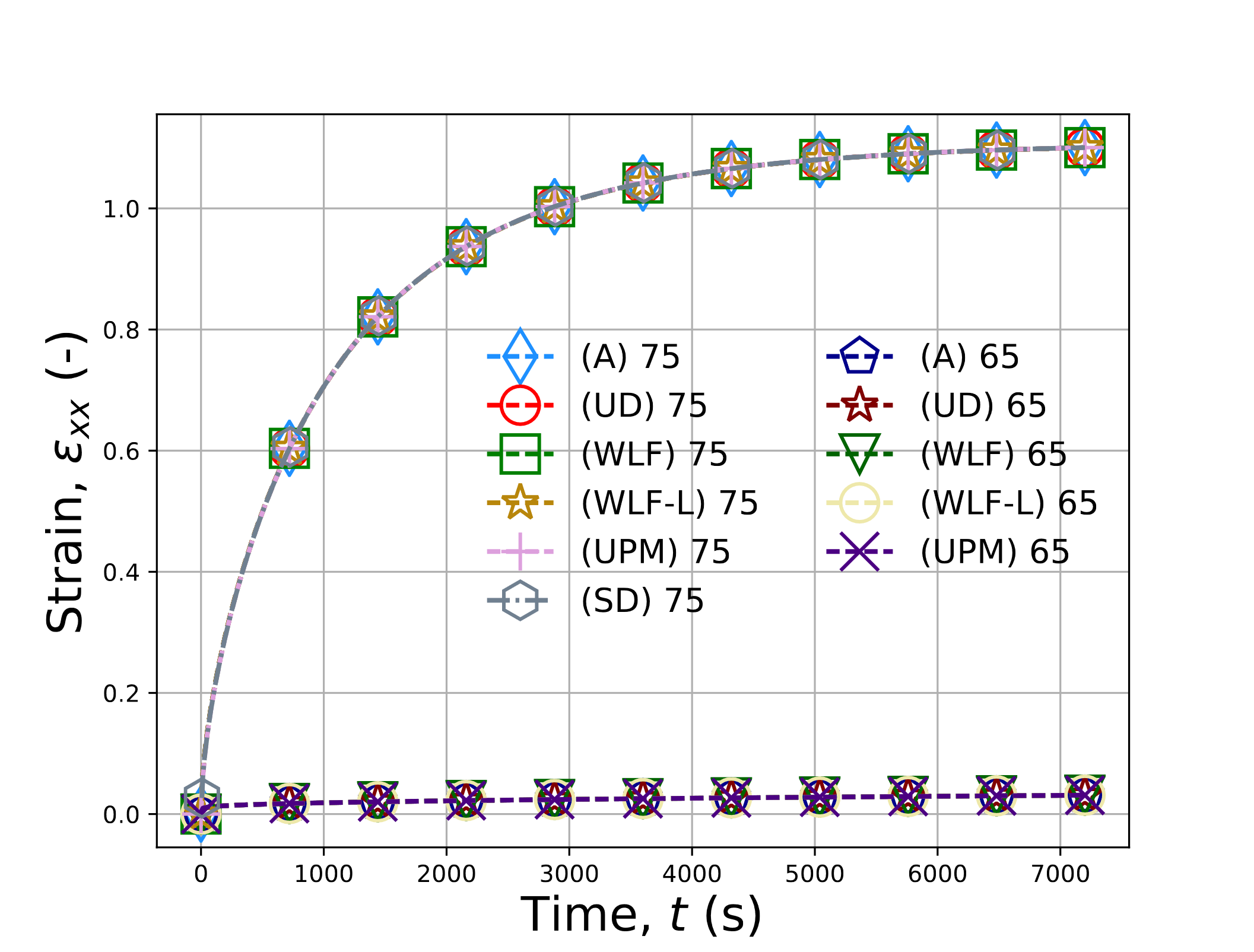
This problem is run with \(\theta\left(t=0\right)=65^{\circ}\)C and \(75^{\circ}\)C and a mechanical load initially at \(\sigma\left(t=0\right)=0\) increasing to 10 MPa in 10 seconds. The load is then held for two hours. To consider the user-defined shift factor, an analytical function of the WLF shift factor is defined and used for the tests. Both the semi-analytic expression of (4.172) and equivalent responses of the LTVE model are considered. As a further test, the UNIVERSAL_POLYMER model is reduced to the same response and is also presented in Fig. 4.140. For a final comparison, the viscoelastic capabilities of Sierra/StructuralDynamics (the Linear Viscoelastic model) are also considered. However, the shift factor form used in that model uses the WLF expression above \(\theta_{\text{ref}}\) and a different expression below. Therefore, results from that model are only given for the case of \(\theta\left(t=0\right)=75^{\circ}\)C case.

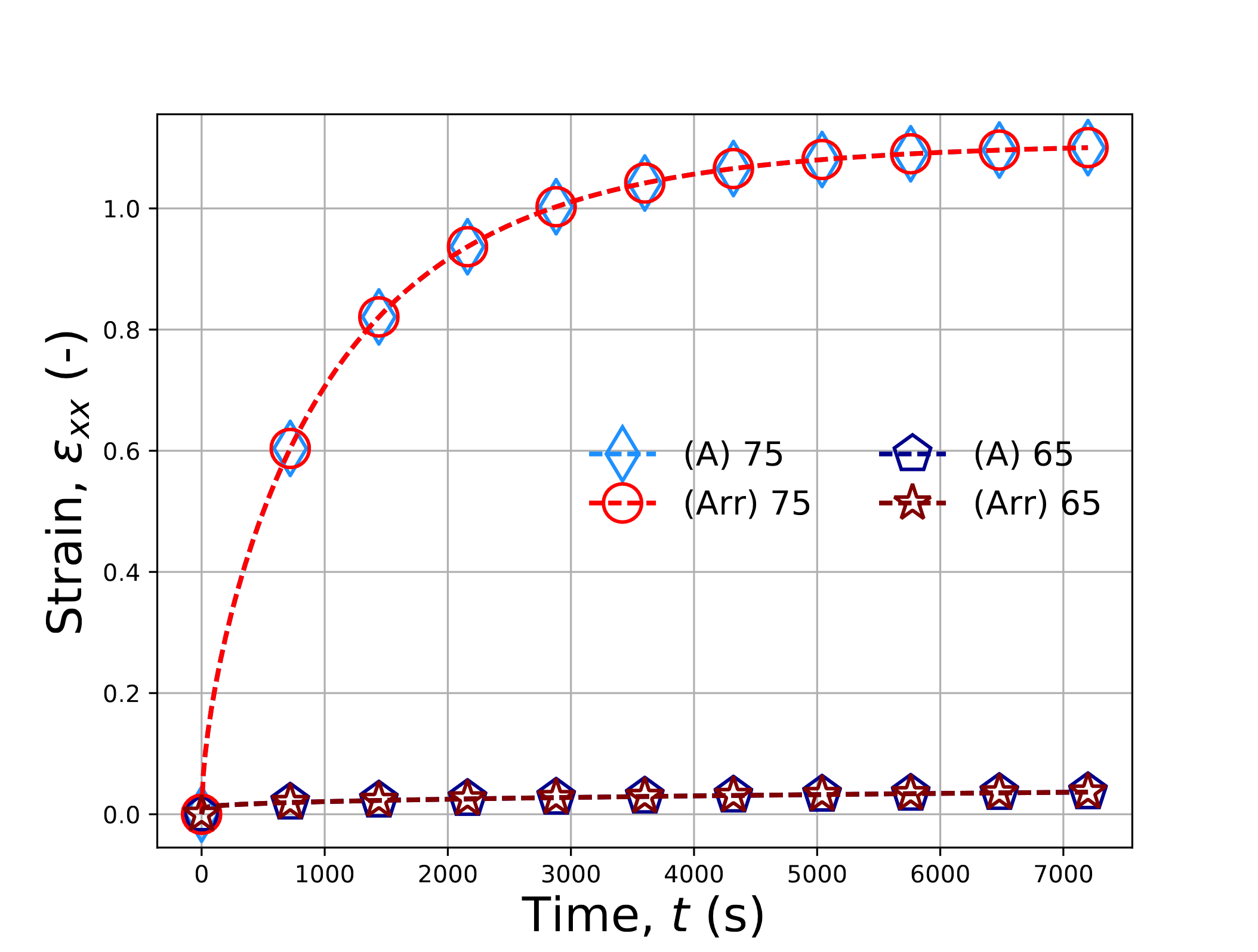
Results for the various WLF shift factor cases are given in Fig. 4.140(a) while Arrhenius shift factors are found in Fig. 4.140(b). In all of the analyses, 1000 time steps are used. In all instance, agreement is observed between all the results.

WLF

Arr

Fig. 4.140 Verification results for the balanced biaxial creep problem for models with (\(a\)) WLF and (\(b\)) Arrhenius shift factors at 65\(^{\circ}\)C and 75\(^{\circ}\)C. Results labelled with (A), (UPM), and (SD) reflect solutions obtained from (4.172), the UNIVERSAL_POLYMER model, and Sierra/SD, respectively. Results from the LTVE model with user-defined, WLF, WLF_LAG, and Arrhenius shift factors are denoted, respectively, (UD), (WLF), (WLF-L), and (Arr).

4.33.3.2. Hydrostatic Creep

As the previous balanced biaxial loading produced a purely deviatoric stress state it correspondingly tested only the deviatoric spectra. To probe the volumetric response, a pure hydrostatic creep test is now investigated. For this purpose, a stress state of the form,

\[\begin{split}\sigma_{ij}\left(t\right) = \frac{1}{3}\left[\begin{array}{ccc} p\left(t\right) & 0 & 0 \\ 0 & p\left(t\right) & 0 \\ 0 & 0 & p\left(t\right) \end{array}\right],\end{split}\]

is assumed. Taking the temperature history to be constant (\(\theta\left(t\right)=\theta\left(t=0\right)\)) yields a stress state of the form,

(4.173)\[\sigma_{ij}=K^{\infty}\varepsilon_{kk}\delta_{ij}+\Delta K J^1\delta_{ij}.\]

Integrating (4.173) implicitly yields the semi-analytical relation,

(4.174)\[\varepsilon_{mm}^{n+1} = \frac{p^{n+1}-3\Delta K\sum_{k=1}^{n_v}w_k^v\frac{a^{n+1}\tau_k^v}{a^{n+1}\tau_k^v+\Delta t}\left(J_n^{1\left(k\right)}-\varepsilon_{mm}^n\right)} {3\left(K^{\infty}+\Delta K\sum_{k=1}^{n_v}w_k^v\frac{a^{n+1}\tau_k^v}{a^{n+1}\tau_k^v+\Delta t}\right)}.\]

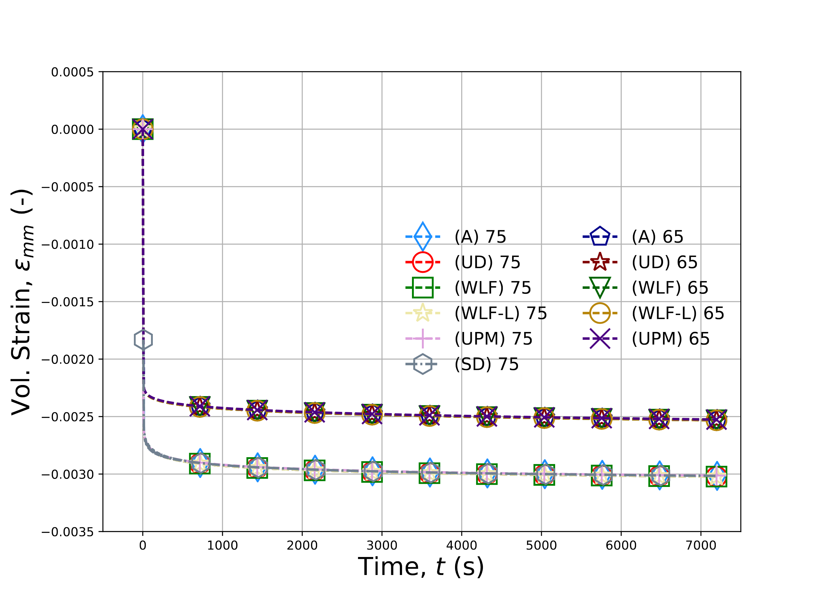
To verify the LTVE model response, the creep problem is solved for temperatures of \(\theta\left(t=0\right)=65^{\circ}\)C and \(75^{\circ}\)C with an applied pressure of -30 MPa applied via a linear ramp over 10 s and then held constant for two hours. 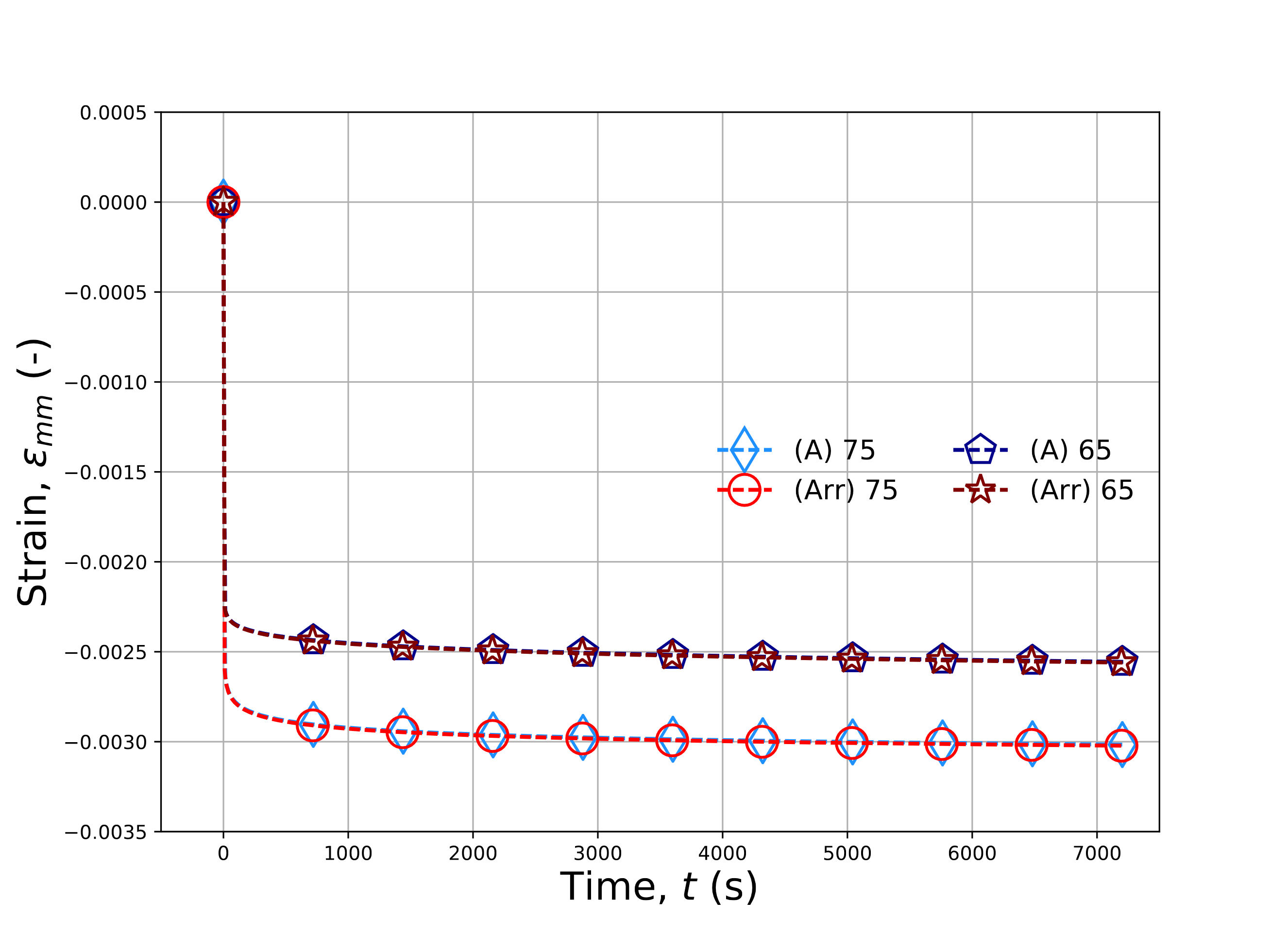Results for the semi-analytical model, LTVE model with the WLF, WLF_LAG (WLF-L), and user-defined (UD) shift factors as well as the UNIVERSAL_POLYMER model at both temperatures as well as the Sierra/StructuralDynamics (SD) response at 75\(^{\circ}\)C are presented in Fig. 4.141(a). Semi-analytical expressions and LTVE results with the Arhhenius shift factor are given in Fig. 4.141(b). In both figures, semi-analytical results are indicated by an \((A)\) and all simulations use 1,000 time steps during the hold portion of the creep loading.

WLF

Arr

Fig. 4.141 Verification results for the hydrostatic creep problem for models with (\(a\)) WLF and (\(b\)) Arrhenius shift factors at 65\(^{\circ}\)C and 75\(^{\circ}\)C. Results labelled with (A), (UPM), and (SD) reflect solutions obtained from (4.174), the UNIVERSAL_POLYMER model, and Sierra/SD, respectively. Results from the LTVE model with user-defined, WLF, WLF_LAG, and Arrhenius shift factors are denoted, respectively, (UD), (WLF), (WLF-L), and (Arr).

From the results in Fig. 4.141, clear agreement is noted across all of the results verifying the implementation of the volumetric hereditary integrals.

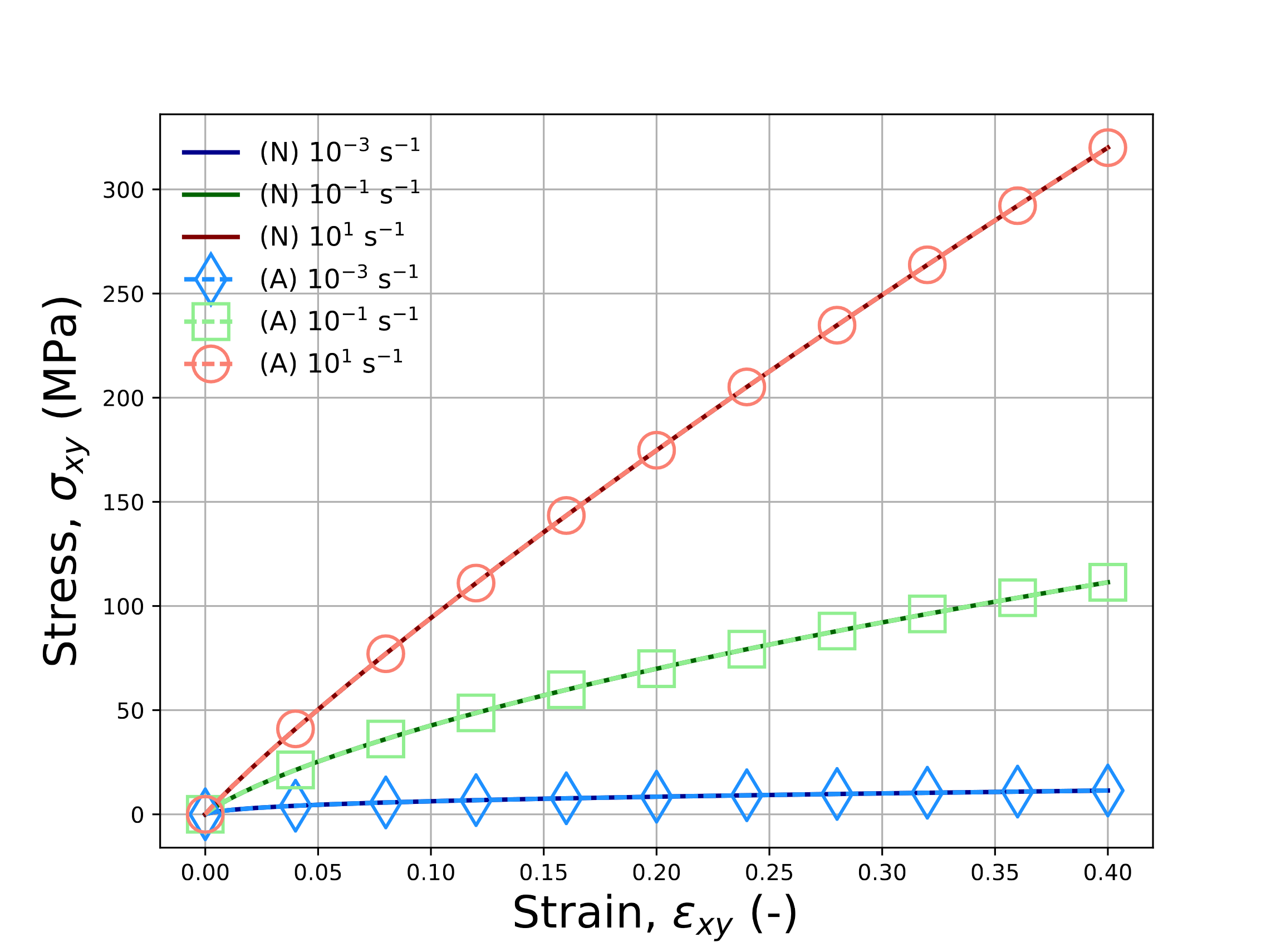
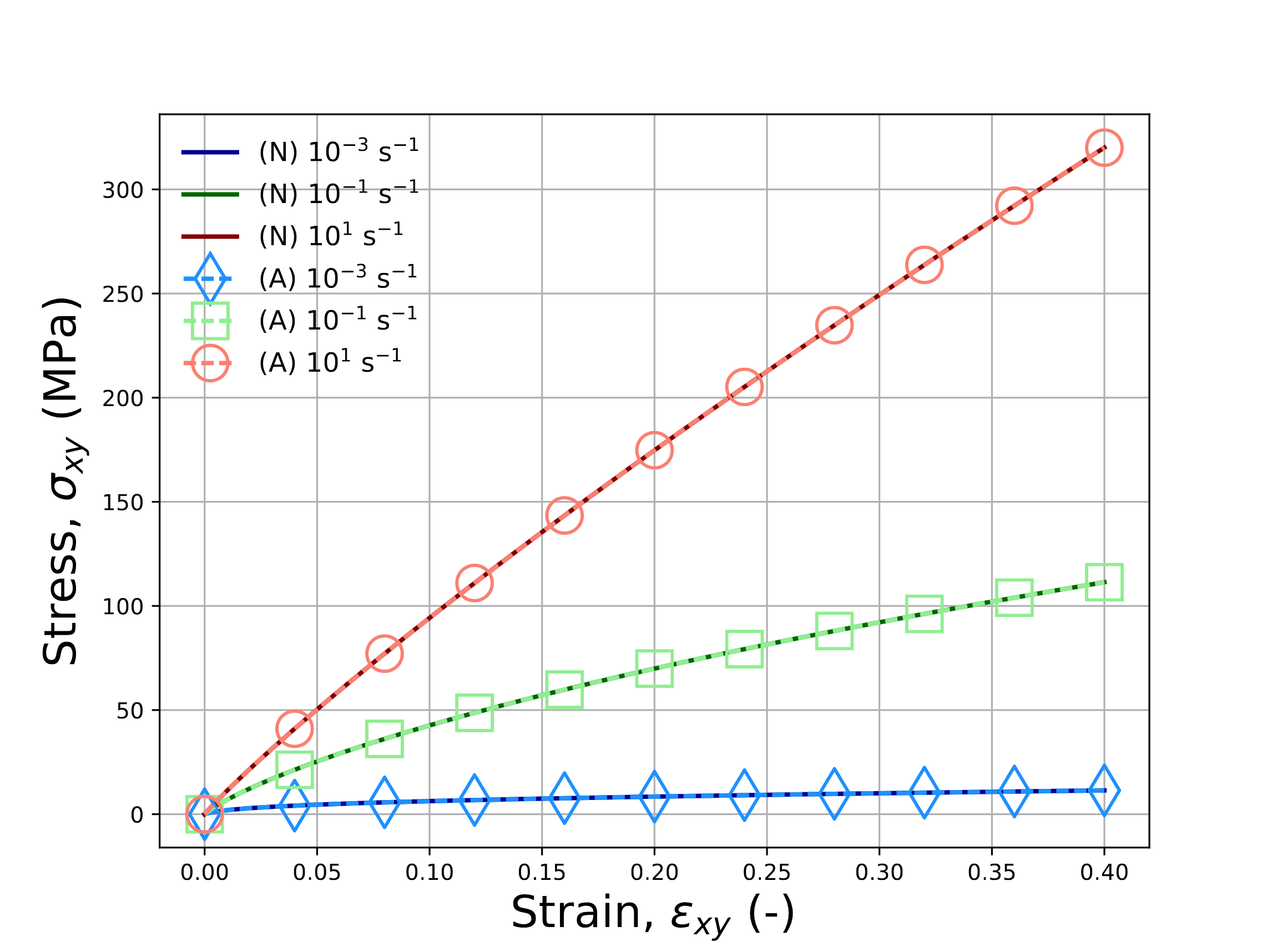
4.33.3.3. Pure Shear

The two prior investigations probed the model response under various creep loadings. Such cases neglect to consider regimes with evolving mechanical loads. Further, while both the volumetric and deviatoric spectra were tested, the resulting stress states only had normal components. Therefore, to test both of these limitations, verification exercises with an isothermal, constant strain rate pure shear mechanical loadings are pursued. For these studies, \(\varepsilon_{xy}\left(t\right)=\dot{\bar{\varepsilon}}t\) and all other strains are zero. With the isothermal profile and pure shear mechanical loadings the volumetric contributions are zero and may be neglected. The only non-zero stress is \(\sigma_{xy}\) which may be described via (4.171). Unlike the previous cases in which the stress was known and the strain found, the current study has a prescribed strain path in which the stress must be determined. Using the previous assumptions and an implicit integration scheme, a semi-analytic expression for the updated stress is given by,

(4.175)\[\sigma_{xy}=2\mu^{\infty}\varepsilon_{xy}^{n+1}+2\Delta\mu\sum_{i=1}^{n_{\text{shear}}}w_k^s\left(\frac{a^{n+1}\tau_k^s}{a^{n+1}\tau_k^s+\Delta t}\right)\left(J_{xy}^{2\left(k\right)\left(n\right)}+\dot{\varepsilon}_{xy}\Delta t\right).\]

To enable comparing the responses across shift factors, the loading is simulated for three different strain rates at \(T\left(t\right)=T_{\text{ref}}=75^{\circ}\)C. Responses are presented for the semi-analytical in (4.175) as well as via the LTVE model with various shift factors and the UNIVERSAL_POLYMER model in Fig. 4.142. For every case presented in Fig. 4.142, agreement is noted across all responses.

WLF

WLF Lag

UD

ARR

UPM

Fig. 4.142 Verification results for the pure shear, constant strain rate problem for LTVE model with (\(a\)) WLF, (\(b\)) WLF_Lag (\(c\)) user-defined (ud), (\(d\)) Arrhenius (Arr) shift factors and (\(e\)) UNIVERSAL_POLYMER model at 75\({\circ}\)C and shear strain rates of \(\dot{\varepsilon}_{xy}=1\times 10^{-3},~1\times 10^{-1}\), and \(1\times 10^{1}\) s\(^{-1}\). Solutions determined through the reduced in (4.175) are (A).

4.33.3.4. No-Load Cooling

All of the previous cases considered isothermal temperature profiles. Differences in the shift factors were introduced via the use of varying constant temperatures and applied strain rates. However, the hereditary integral in the WLF_Lag shift factor does not play a role in such cases and therefore is not tested. To alleviate this, a no-load cooling profile is investigated. Specifically, a problem previously considered in [[7]] is studied here. It consists of cooling a representative inorganic glass (Schott 8061) extensively characterized by Chambers et al. [[8]] from 510\(^{\circ}\)C (\(T_{\text{ref}}+50^{\circ}\)C) to 150\(^{\circ}\)C (783 K to 423K) at different constant cooling rates. The model parameterizations used in this study may be found in corresponding references [[7], [8]] and are not repeated here for brevity (for the Arrhenius shift factor, a value of \(E_a/R=23,670\) was found by doing a best fit to the WLF expression). For this test, temperature dependence of thermoelastic constants is neglected to simplify the restrict the impact of cooling to the shift factor. A constant cooling rate of \(\dot{T}=2^{\circ}\)C/min is used for all shift factors while additional rates of \(\dot{T}=0.2\) and \(20^{\circ}\)C/min are also used to assess history dependence.

By implicitly integrating \(J^1\) and noting that the response is purely volumetric, an expression for the volume strain may be given as,

(4.176)\[\begin{split}\varepsilon_{kk}^{n+1} = & \frac{1}{K^{\infty}+\Delta K\sum_{i=1}^{n_{\text{bulk}}}\frac{a^{n+1}\tau_k^v}{a^{n+1}\tau_k^v+\Delta t}} \left[3K^{\infty}\alpha^{\infty}\left(T-T_0\right)+3\Delta\left(\alpha K\right)J_{n+1}^3\right. \nonumber \\ & \left.-\Delta K\sum_{i=1}^{n_{\text{bulk}}}\frac{a^{n+1}\tau_k^v}{a^{n+1}\tau_k^v+\Delta t}\left(J_n^{1\left(k\right)}-\varepsilon_{kk}^n\right)\right].\end{split}\]

The previous relation assumes that \(J_{n+1}^3\) is known. As this term is purely temperature and history dependent it may be integrated seperately knowing the loading history. For the WLF_Lag shift factor this is a non-linear relation. Regardless, for all cases of interest this term is found via implicit integration.

Fig. 4.143 presents results determined semi-analytically via (4.176) and numerically via the LTVE model. Histories for the (\(a\)) log\(_{10}a\) (\(b\)) \(\varepsilon_{kk}\) (\(c\)) \(J^1\) and (\(d\)) \(J^3\) are presented for all of the shift factors without history dependence. Good agreement is noted across all results.

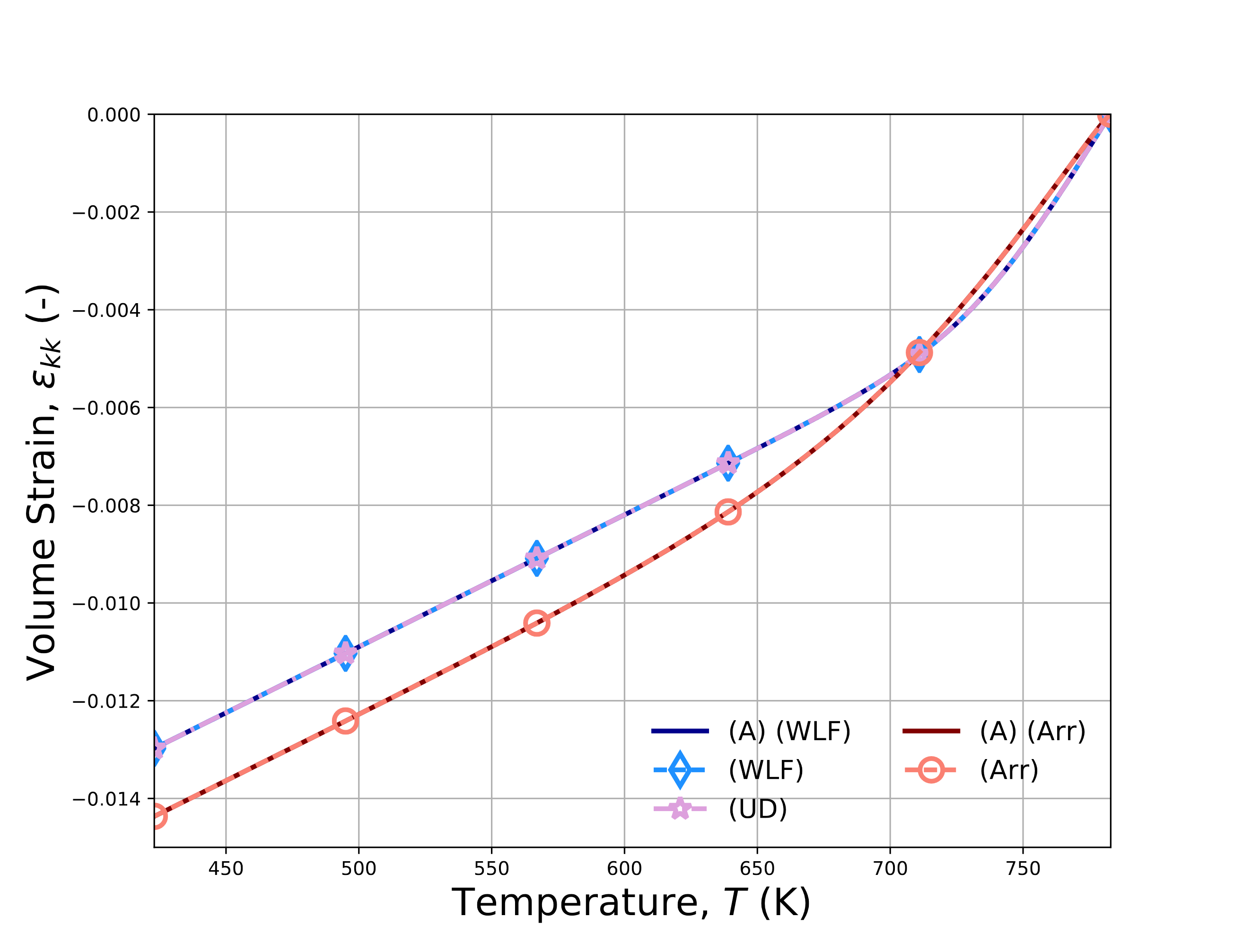
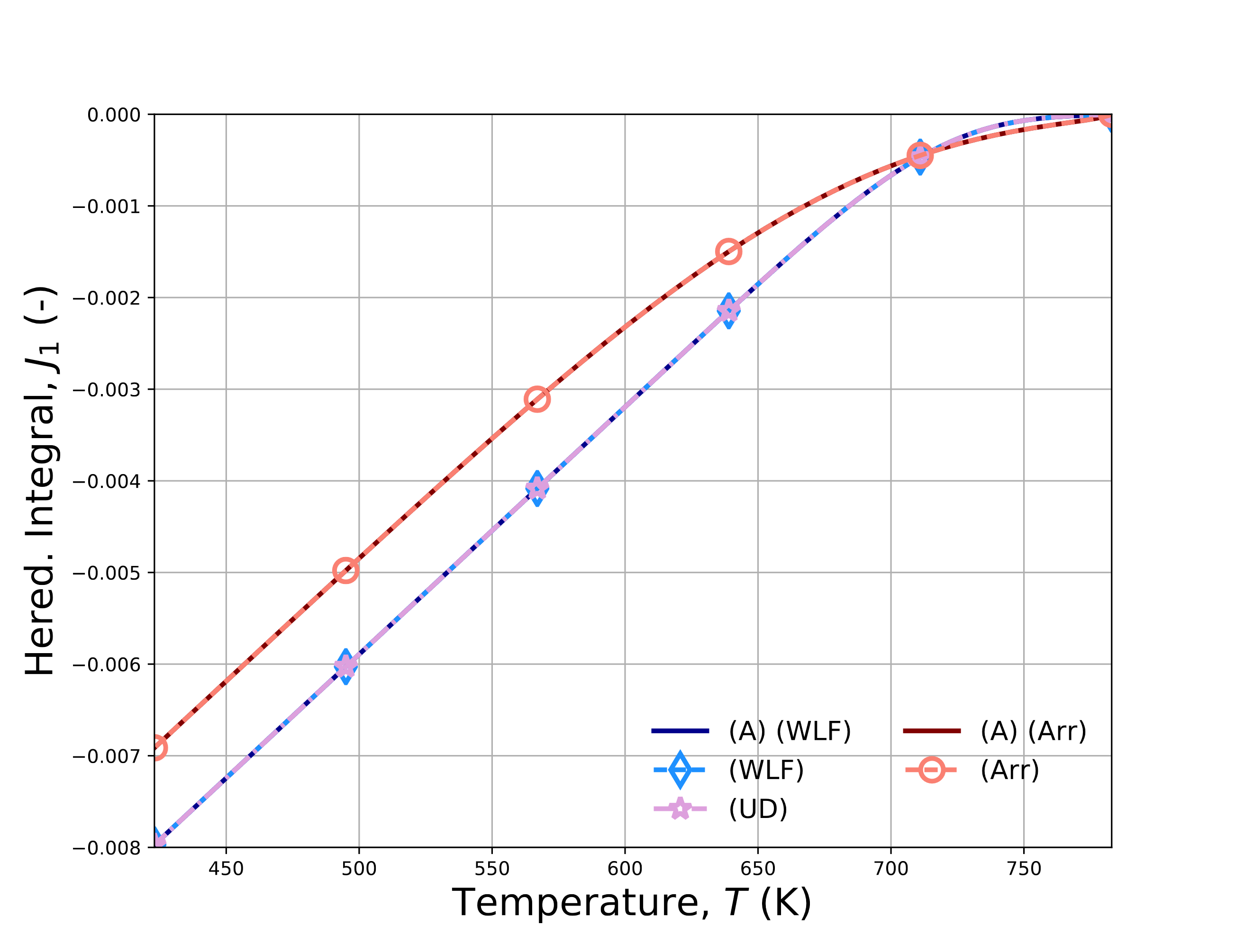
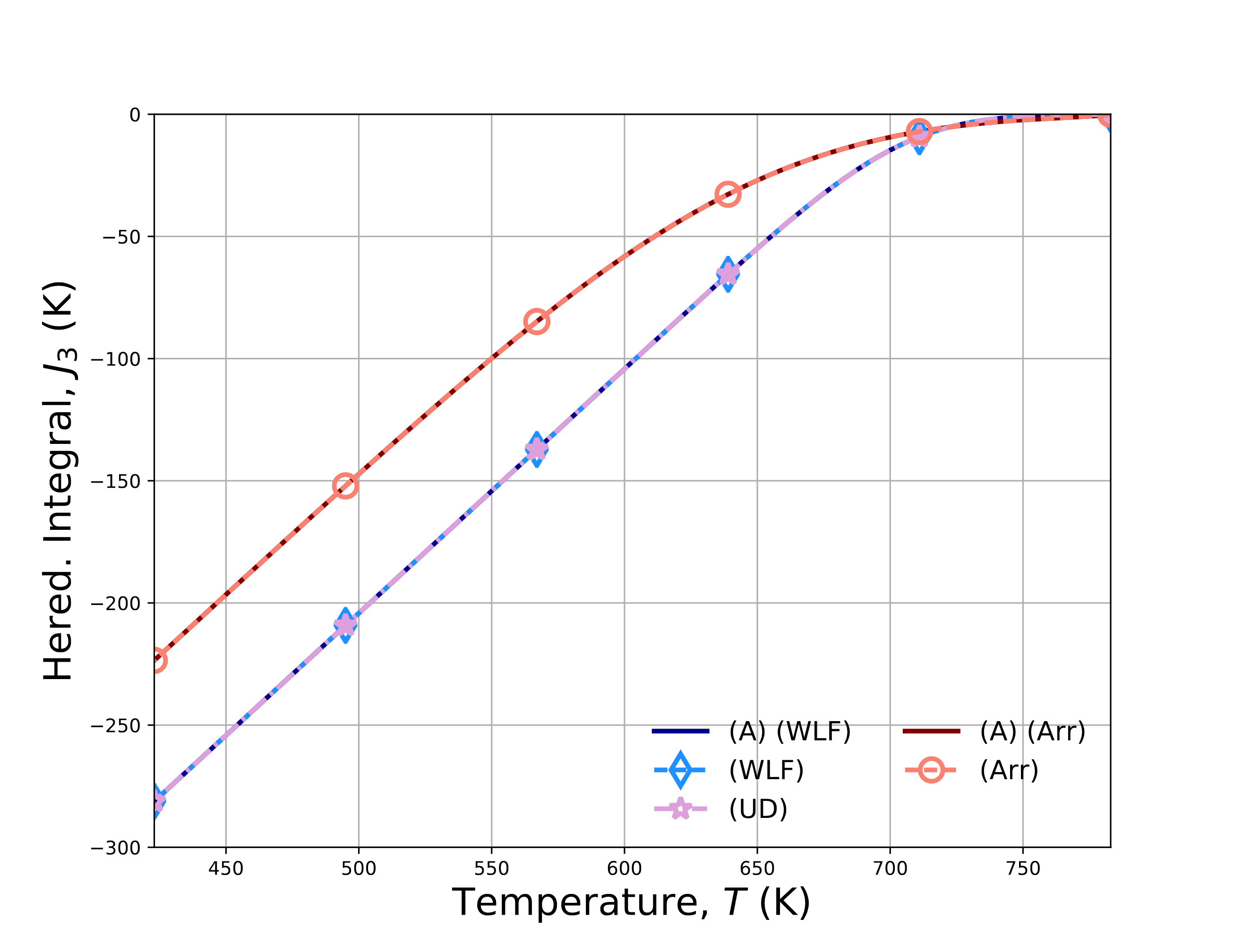
Fig. 4.143 Verification results for the no-load cooling problem for the LTVE model exhibiting analytical and numerical results for (\(a\)) log\(_{10}a\), (\(b\)) \(\varepsilon_{kk}\), (\(c\)) \(J^1\), and (\(d\)) \(J^3\). Results are obtained (A) semi-analytically and with WLF, (UD) user-defined, and (Arr) Arrhenius shift factors.

To consider the impact of the history dependence, results at the three different cooling rates are determined semi-analytically (A), numerically with the LTVE model (N), and numerically with the UNIVERSAL_POLYMER model (UPM) in Fig. 4.144. Evolutions for (\(a\)) log\(_{10}a\) (\(b\)) volume strain (\(c\)) \(J_1\) and (\(d\)) \(J_3\). The \(J_1\) and \(J_3\) results are not presented for the UPM case as they are not readily output. Once more, good agreement is noted across all of the results.

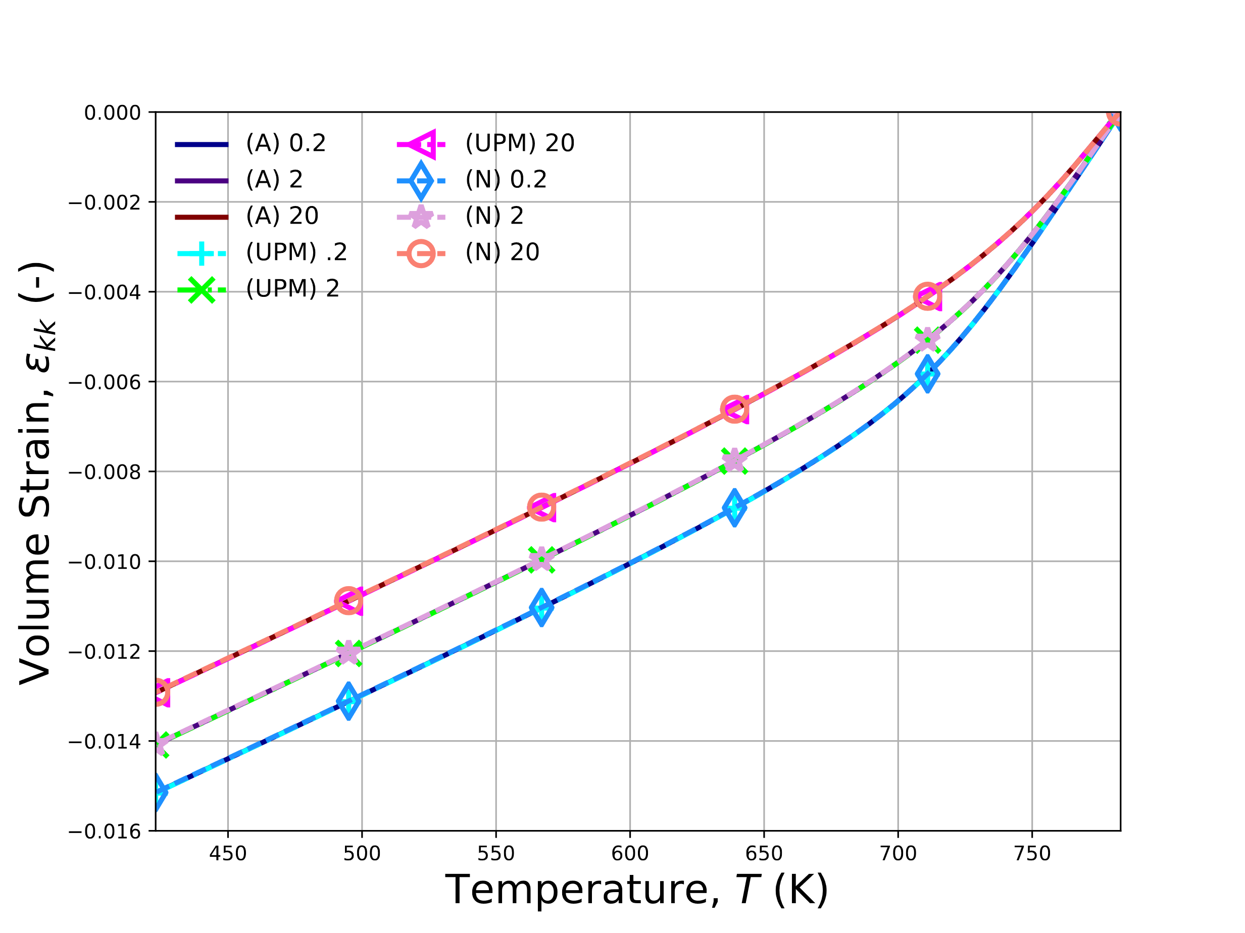
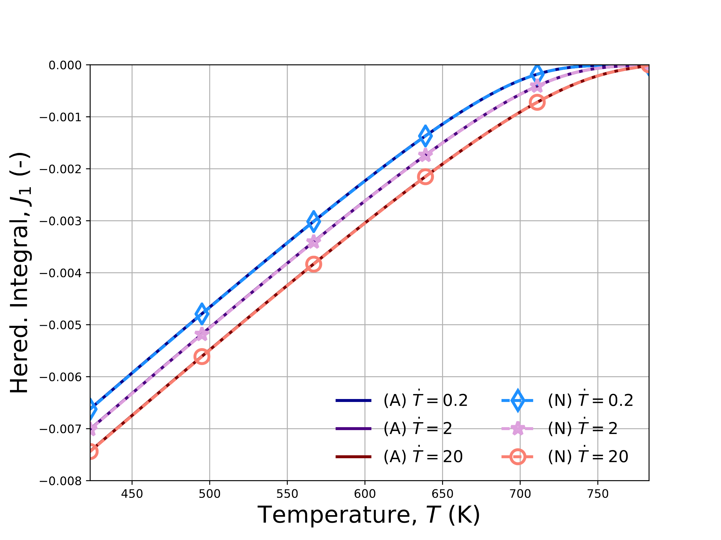
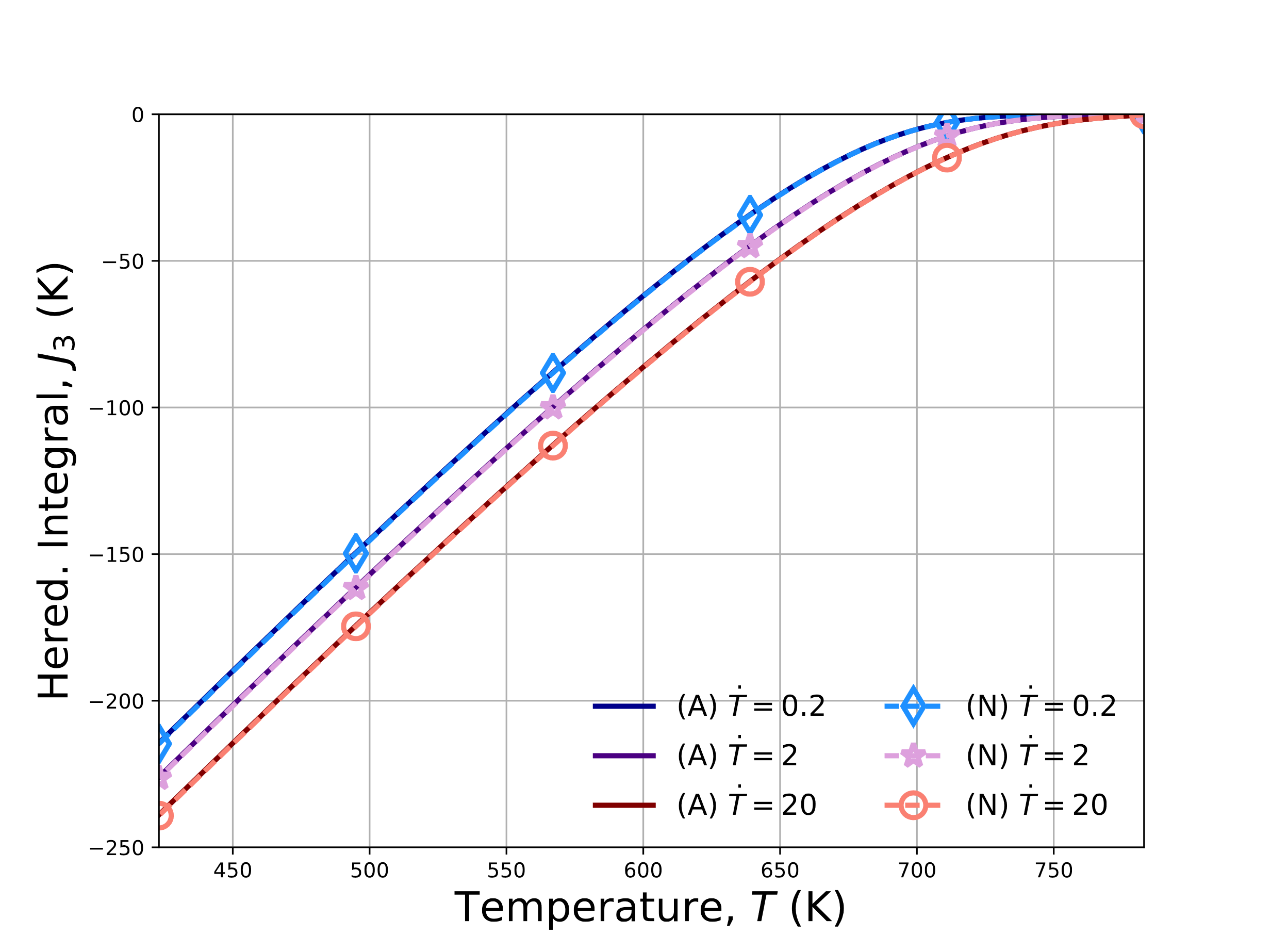
Fig. 4.144 Verification results for the no-load cooling problem for the LTVE and UNIVERSAL_POLYMER models exhibiting analytical and numerical results for (\(a\)) log\(_{10}a\), (\(b\)) \(\varepsilon_{kk}\), (\(c\)) \(J^1\), and (\(d\)) \(J^3\). The numbers in the legend indicate cooling rates of \(\dot{T}=0.2,~2,\) and \(20\) K/min and results are obtained semi-analytically (A), numerically with the LTVE model (N), and numerically with the UNIVERSAL_POLYMER (UPM) model.

4.33.4. User Guide

BEGIN PARAMETERS FOR MODEL LINEAR_THERMOVISCOELASTIC
  #
  SHEAR MODULUS  = <real>
  BULK MODULUS   = <real>
  #
  BULK RUBBERY 0  = <real>
  SHEAR RUBBERY 0 = <real>
  ALPHA RUBBERY 0 = <real>
  #
  BULK GLASSY 0  = <real>
  SHEAR GLASSY 0 = <real>
  ALPHA GLASSY 0 = <real>
  #
  #  - Optional temperature dependence of thermoelastic constants
  #
  BULK RUBBERY TEMPERATURE DEPENDENCE  = <string>
  SHEAR RUBBERY TEMPERATURE DEPENDENCE = <string>
  ALPHA RUBBERY TEMPERATURE DEPENDENCE = <string>
  #
  BULK GLASSY TEMPERATURE DEPENDENCE  = <string>
  SHEAR GLASSY TEMPERATURE DEPENDENCE = <string>
  ALPHA GLASSY TEMPERATURE DEPENDENCE = <string>
  #
  #  - Reference temperature only needed
  #    if using temperature dependent parameters
  #
  T0 = <real>
  #
  SHIFT FACTOR MODEL = WLF | ARRHENIUS | USER_DEFINED | WLF_LAG
  #
  #  - IF SHIFT FACTOR MODEL = WLF | WLF_LAG
  #
  WLF C1 = <real>
  WLF C2 = <real>
  REFERENCE TEMPERATURE   = <real>
  #
  #  - IF SHIFT FACTOR MODEL = ARRHENIUS
  #
  NORM ACTIVATION ENERGY = <real>
  REFERENCE TEMPERATURE  = <real>
  #
  #  - IF SHIFT FACTOR MODEL = USER_DEFINED
  #
  SHIFT FACTOR FUNCTION = <string>
  #
  NUM BULK PRONY TERMS = <int>
  #
  BULK RELAX TIME 1 = <real>
  BULK RELAX TIME 2 = <real>
  # ...
  BULK RELAX TIME 30 = <real>
  #
  f1 1  = <real>
  f1 2  = <real>
  # ...
  f1 30 = <real>
  #
  NUM SHEAR PRONY TERMS = <int>
  #
  SHEAR RELAX TIME 1 = <real>
  SHEAR RELAX TIME 2 = <real>
  # ...
  SHEAR RELAX TIME 30 = <real>
  #
  f2 1  = <real>
  f2 2  = <real>
  # ...
  f2 30 = <real>
  #
 END [PARAMETERS FOR MODEL LINEAR_THERMOVISCOELASTIC]

In the command blocks that define the LINEAR_THERMOELASTIC model:

• The bulk and shear moduli of the equilibrium (rubbery) phase are defined by the BULK RUBBERY 0 and SHEAR RUBBERY 0 command lines, respectively.

• The bulk and shear moduli of the glassy phase are defined by the BULK GLASSY 0 and SHEAR GLASSY 0 command lines, respectively.

• The linear coefficients of thermal expansion of the rubbery and glassy phases are given by the ALPHA RUBBERY 0 and ALPHA GLASSY 0 command lines, respectively. Note, the UNIVERSAL POLYMER model uses volumetric – not linear – coefficients of thermal expansion.

• The shift factor model is specified via the SHIFT FACTOR MODEL command line.

• For the WLF or WLF_LAG shift factor models, the \(C_1\) coefficient, \(C_2\) coefficient, and reference temperature, \(\theta_{\text{ref}}\), are defined via the WLF C1, WLF C2, and REFERENCE TEMPERATURE command lines.

• For the Arrhenius shift factor model, the normalized activation energy, \(E_a/R\), and reference temperature, \(\theta_{\text{ref}}\), are specified via the NORM ACTIVATION ENERGY and REFERENCE TEMPERATURE command lines.

• For the user-defined shift factor model, the function name is specified via the SHIFT FACTOR FUNCTION command line. Note, any Sierra scope function may be defined and should be specified as a function of temperature. It is also emphasized the actual shift factor – not the logarithm of it – should be directly defined. Care should be taken to ensure the function is defined and admissible over the expected temperature domain.

• The number of terms in the Prony series of the bulk, \(n_{\text{bulk}}\), and shear, \(n_{\text{shear}}\), are given by the NUM BULK PRONY TERMS and NUM SHEAR PRONY SERIES command lines. These two numbers do not need to be the same and must both be defined. The maximum permissible number is 30 although any lower number is permissible.

• The bulk relaxation spectrum is characterized by a series of times, \(\tau_k^v\), and weights, \(w_k^v\). The times are defined via BULK RELAX TIME 1 through BULK RELAX TIME \(k\) where \(k\) is the number of terms in the spectrum. The same times do not need to be used for the bulk and shear terms. Weights are defined via the f1 1 through f1 \(k\) command lines. \(k\) should be equal to \(n_{\text{bulk}}\).

• The shear relaxation spectrum is characterized by a series of times, \(\tau_k^s\), and weights, \(w_k^s\). The times are defined via SHEAR RELAX TIME 1 through SHEAR RELAX TIME \(k\) where \(k\) is the number of terms in the spectrum. The same times do not need to be used for the bulk and shear terms. Weights are defined via the f2 1 through f2 \(k\) command lines. \(k\) should be equal to \(n_{\text{shear}}\).

Output variables available for this model are listed in Table 4.55. Note, for each of the various hereditary integral individual components may be output by specifying a hereditary integral ..._X where X is an integer term in the spectrum. For instance, the 7\(^{th}\) term of the Prony series of the volume strain integral (\(J^1_7\)) is output by specifying J1_7.

Table 4.55 State Variables for LINEAR_THERMOVISCOELASTIC Model

Name	Description
a	shift factor, \(a\)
J1	volume strain hereditary integral, \(J^1\)
J2_XX	XX component of the deviatoric hereditary integral, \(J^2_{11}\)
J2_YY	YY component of the deviatoric hereditary integral, \(J^2_{22}\)
J2_ZZ	ZZ component of the deviatoric hereditary integral, \(J^2_{33}\)
J2_XY	XY component of the deviatoric hereditary integral, \(J^2_{12}\)
J2_YZ	YZ component of the deviatoric hereditary integral, \(J^2_{23}\)
J2_ZX	ZX component of the deviatoric hereditary integral, \(J^2_{31}\)
J3	thermal strain hereditary integral, \(J^3\)

---

[1]

R.M. Christensen. Theory of Viscoelasticity. Dover Publications, Inc., Mineola, NY, second edition, 2003.

[2] (1,2)

J. M. Caruthers, D. B. Adolf, R. S. Chambers, and P. Shrikhande. A thermodynamically consistent, nonlinear viscoelastic approach for modeling glassy polymers. Polymer, 45:4577–4597, 2004.

[3]

D. B. Adolf, R. S. Chambers, and M. A. Neidigk. A simplified potential energy clock model for glassy polymers. Polymer, 50:4257–4269, 2009.

[4]

M.L. Williams, R.F. Landel, and J.D. Ferry. The temperature dependence of relaxation mechanisms in amorphous polymers and other glass-forming liquids. Journal of the American Chemical Society, 77:3701–3707, 1955.

[5]

B.T. Lester and K.N. Long. Modular linear thermoviscoelastic model. Memo to distribution SAND2020-4973R, Sandia National Laboratories, Albuquerque, NM and Livermore, CA, 2020.

[6]

R.J. Kuether. Two-tier model reduction of viscoelastically damped finite element models. Computers and Structures, 219:58–72, 2019.

[7] (1,2)

B.T. Lester and K.N. Long. Numerical integration of viscoelastic models. Memo to distribution SAND2019-11472R, Sandia National Laboratories, Albuquerque, NM and Livermore, CA, 2019.

[8] (1,2)

R. Chambers, R. Tandon, and M. Stavig. Characterization and calibration of a viscoelastic simplified potential energy clock model for inorganic glasses. Journal of Non-Crystalline Solids, 432:545–555, 2016.