4.4. Elastic Three Dimensional Orthotropic Model

4.4.1. Theory

The ELASTIC 3D ORTHOTROPIC model is an extension of the previously discussed ELASTIC routine and describes the linear elastic response of a material which exhibits orthotropic symmetry, where the orientation of the principal material directions can be arbitrary with respect to the global Cartesian axes as specified by the user.

First, a rectangular, cylindrical, or spherical reference coordinate system is defined. The material coordinate system can then be defined through two successive rotations about axes in the reference coordinate system. These principal axes are denoted as A, B, and C in the following. Thermal strains are also defined with respect to these principal material axes.

The elastic stiffness for an orthotropic material can be described in terms of the elastic compliance which relates the strain to the stress, \(\varepsilon_{ij} = \mathbb{S}_{ijkl}\sigma_{kl}\). For a material with an orthogonal ABC coordinate system, and written in that reference frame, the elastic compliance tensor is given by

(4.5)\[\begin{split}\left[ \tilde{\mathbb{S}} \right] = \begin{bmatrix} \frac{1}{E_{AA}} & -\frac{\nu_{BA}}{E_{BB}} & -\frac{\nu_{CA}}{E_{CC}} & 0 & 0 & 0 \\ \\ -\frac{\nu_{AB}}{E_{AA}} & \frac{1}{E_{BB}} & -\frac{\nu_{CB}}{E_{CC}} & 0 & 0 & 0 \\ \\ -\frac{\nu_{AC}}{E_{AA}} & -\frac{\nu_{BC}}{E_{BB}} & \frac{1}{E_{CC}} & 0 & 0 & 0 \\ \\ 0 & 0 & 0 & \frac{1}{2G_{AB}} & 0 & 0 \\ \\ 0 & 0 & 0 & 0 & \frac{1}{2G_{BC}} & 0 \\ \\ 0 & 0 & 0 & 0 & 0 & \frac{1}{2G_{CA}} \end{bmatrix},\end{split}\]

where the \(~\tilde{\cdot}~\) is used to denote a variable in the \(ABC\) material system.

From the definition (4.5), it can be seen that requiring symmetry leads to relations of the form,

\[\nu_{BA} = \nu_{AB}\frac{E_{BB}}{E_{AA}} \;\;\; ; \;\;\; \nu_{CB} = \nu_{BC}\frac{E_{CC}}{E_{BB}} \;\;\; ; \;\;\; \nu_{AC} = \nu_{CA}\frac{E_{AA}}{E_{CC}}.\]

Therefore, only 9 independent constants are needed to fully define the model behavior.

The orthotropic model is also formulated in a hypoelastic fashion, leading to a constitutive equation (in the ABC material frame) of,

\[\stackrel{\circ}{\tilde{\sigma}}_{ij} = \tilde{\mathbb{C}}_{ijkl}\left(\tilde{D}_{kl}-\tilde{D}^{th}_{kl}\right),\]

where \(\tilde{D}^{th}_{ij}\) is the thermal strain rate.

The elastic stiffness tensor, \(\tilde{\mathbb{C}}_{ijkl}\), is the inverse of the compliance, \(\tilde{\mathbb{C}}_{ijkl} = \tilde{\mathbb{S}}_{ijkl}^{-1}\), and as such may be determined to be,

\[\begin{split}\left[ \tilde{\mathbb{C}} \right] = \begin{bmatrix} \mathbb{C}_{AAAA} & \mathbb{C}_{AABB} & \mathbb{C}_{CCAA} & 0 & 0 & 0 \\ \\ \mathbb{C}_{AABB} & \mathbb{C}_{BBBB} & \mathbb{C}_{BBCC} & 0 & 0 & 0 \\ \\ \mathbb{C}_{CCAA} & \mathbb{C}_{BBCC} & \mathbb{C}_{CCCC} & 0 & 0 & 0 \\ \\ 0 & 0 & 0 & 2G_{AB} & 0 & 0 \\ \\ 0 & 0 & 0 & 0 & 2G_{BC} & 0 \\ \\ 0 & 0 & 0 & 0 & 0 & 2G_{CA} \end{bmatrix}.\end{split}\]

where

\[\begin{split}\mathbb{C}_{AAAA} & = \frac{1-\nu_{BC}\nu_{CB}}{\Delta}E_{AA} \;\;\; ; \;\;\; \mathbb{C}_{BBBB} = \frac{1-\nu_{CA}\nu_{AC}}{\Delta}E_{BB} \;\;\; ; \;\;\; \mathbb{C}_{CCCC} = \frac{1-\nu_{AB}\nu_{BA}}{\Delta}E_{CC} \nonumber \\ \mathbb{C}_{AABB} & = \frac{\nu_{BA}+\nu_{CA}\nu_{BC}}{\Delta}E_{AA} \;\;\; ; \;\;\; \mathbb{C}_{BBCC} = \frac{\nu_{CB}+\nu_{AB}\nu_{CA}}{\Delta}E_{BB} \;\;\; ; \;\;\; \mathbb{C}_{CCAA} = \frac{\nu_{AC}+\nu_{BC}\nu_{AB}}{\Delta}E_{CC} \nonumber\end{split}\]

and \(\Delta = 1 - \nu_{AB}\nu_{BA} - \nu_{BC}\nu_{CB} - \nu_{CA}\nu_{RT} - 2\nu_{AB}\nu_{BC}\nu_{CA}\).

[[1]] for more information about the elastic three-dimensional orthotropic model.

4.4.2. Implementation

Given the similarities in formulation, the 3D orthotropic and elastic models are integrated in a similar fashion. Section 4.3.2 discussed many of these issues in detail for the isotropic elastic formulation. As such, in this section, special attention is paid to the treatment of the complexity associated with the orthotropic model – namely, the multiple coordinate systems.

To implement the elastic 3D orthotropic model, two coordinate systems need to be considered – the local \(ABC\) material and global \(XYZ\) coordinate systems. The former is used in defining the material response and the latter refers to the larger boundary value problem being analyzed. To map between these configurations, a user-defined coordinate system is specified that can be rotated twice about one of its current axes to give the final, desired directions. A corresponding rotation tensor, \(\tilde{Q}_{ij}\), may also be constructed in this way and used to transform various variables. Noting that the elastic stiffness tensor is constant throughout loading enables the transformation

(4.6)\[\mathbb{C}_{ijkl}~=~\tilde{Q}_{ai}\tilde{Q}_{bj}\tilde{Q}_{ck}\tilde{Q}_{dl}\tilde{\mathbb{C}}_{abcd}\]

to be performed during initialization. The \(~\tilde{\cdot}~\) is used with the rotation tensor \(Q_{ij}\) to emphasize that it does not map between the unrotated and rotated configurations (as defined in (4.1)) and is instead associated with transforming between the \(ABC\) and \(XYZ\) frames.

In the material coordinate system, the thermal strain tensor may be written as,

\[\tilde{\varepsilon}^{th}_{ij}~=~\varepsilon^{th}_{aa}\left(\theta\right)\delta_{ia}\delta_{ja}+\varepsilon^{th}_{bb}\left(\theta\right)\delta_{ib}\delta_{jb}+\varepsilon^{th}_{cc}\left(\theta\right)\delta_{ic}\delta_{jc},\]

where \(\varepsilon^{th}_{aa}\left(\theta\right),~\varepsilon^{th}_{bb}\left(\theta\right),\) and \(\varepsilon^{th}_{cc}\left(\theta\right)\) are the temperature (\(\theta\)) dependent thermal strain functions in the \(A,~B,\) and \(C\) principal material directions, respectively, and \(\delta_{ij}\) is the Kronecker delta. Using the same constant transformation, \(\tilde{Q}_{ij}\), the \(XYZ\)-system thermal strain tensor is determined to be,

(4.7)\[\varepsilon^{th}_{ij}\left(\theta\right)~=~\tilde{Q}_{ai}\tilde{\varepsilon}^{th}_{ab}\tilde{Q}_{jb}.\]

Following (4.3), the updated Cauchy stress may then be found to be,

\[\sigma^{n+1}_{ij}=R^{n+1}_{ik}R^n_{mk}\sigma^n_{mn}R^n_{nl}R^{n+1}_{jl}+\mathbb{C}_{ijkl}\left(\Delta tD_{kl}-\left(\varepsilon^{th}_{kl}\left(\theta^{n+1}\right)-\varepsilon^{th}_{kl}\left(\theta^n\right)\right)\right),\]

where the time dependency in the thermal strains is accounted for through changes in the temperature field.

4.4.3. Verification

The elastic 3D orthotropic model is verified through both biaxial displacement and uniaxial strain tests. The first is performed with the material and global coordinate systems aligned to investigate anisotropy while the second is done with the material coordinate system misaligned with respect to the global system. The latter also incorporates a thermal loading component to test the thermal strain contributions. In this case, it is assumed that each of the thermal strain input functions have linear slopes of \(\alpha_{aa},~\alpha_{bb},\) and \(\alpha_{cc}\) for the \(A,~B,\) and \(C\) principal material axes, respectively. A common zero strain reference temperature, \(T_0\), is assumed for all three functions. The set of material properties used for these tests are given in Table 4.1.

Table 4.1 The material properties for the elastic 3D orthotropic model used for the varying temperature, uniaxial stress tests.

\(E_{AA}=E\)	10,000.0 ksi	\(G_{AB}\)	100.0 ksi
\(E_{BB}\)	200.0 ksi	\(G_{BC}\)	1,000.0 ksi
\(E_{CC}\)	10.0 ksi	\(G_{CA}\)	5.0 ksi
\(\nu_{AB} = \nu\)	0.25	\(\alpha_{aa}\)	50 \(\frac{\mu\varepsilon}{\text{K}}\)
\(\nu_{BC}\)	0.2	\(\alpha_{bb}\)	500 \(\frac{\mu\varepsilon}{\text{K}}\)
\(\nu_{CA}\)	0.003	\(\alpha_{cc}\)	5 \(\frac{\mu\varepsilon}{\text{K}}\)
		\(\theta_0\)	293 K

4.4.3.1. Biaxial Displacement

First, to investigate anisotropic effects, the case of a biaxial applied displacement of the form,

\[u_i=\lambda_1\delta_{1i}+\lambda_2\delta_{2i},\]

is considered for a material which has its axes aligned with the global Cartesian system – \(\alpha_1=\alpha_2=0\) or the \(A,~B,\) and \(C\) frame is the same as the \(\hat{\text{e}}_1,~\hat{\text{e}}_2,\) and \(\hat{\text{e}}_3\). To simplify the problem, \(\lambda_2=\frac{1}{2}\lambda_1\) and it can be shown that (noting \(\sigma_{33}=0\) from a corresponding traction free condition),

\[\begin{split}\varepsilon_{11} = & \ln\left(1+\lambda_1\right), \nonumber \\ \varepsilon_{22} = & \ln\left(1+\frac{1}{2}\lambda_1\right) \nonumber \\ \varepsilon_{33} = & -\frac{\nu_{AC}+\nu_{BC}\nu_{AB}}{1-\nu_{AB}\nu_{BA}}\varepsilon_{11} -\frac{\nu_{BC}+\nu_{BA}\nu_{AC}}{1-\nu_{AB}\nu_{BA}}\varepsilon_{22}.\end{split}\]

With the strain state known, analytical stresses may be found via Hooke’s law. The corresponding results of both the numerical and analytical results are presented below in Fig. 4.6. Numerical results are found through a single element test. Importantly, by comparing the results of Fig. 4.6(a) and Fig. 4.6(b) the expected and desired anisotropy may be clearly seen in the vast difference of stress magnitudes (as indicated by the figure scaling). Additionally, the matching results serves to verify the model under such conditions.

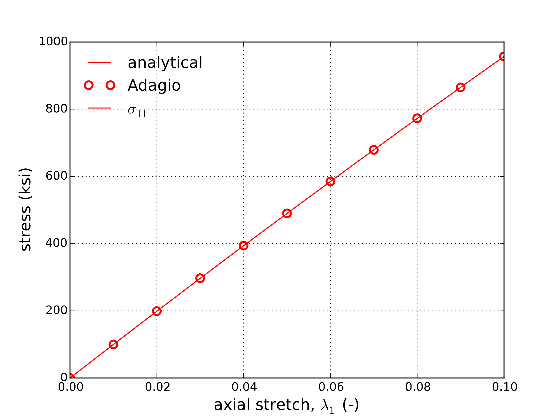
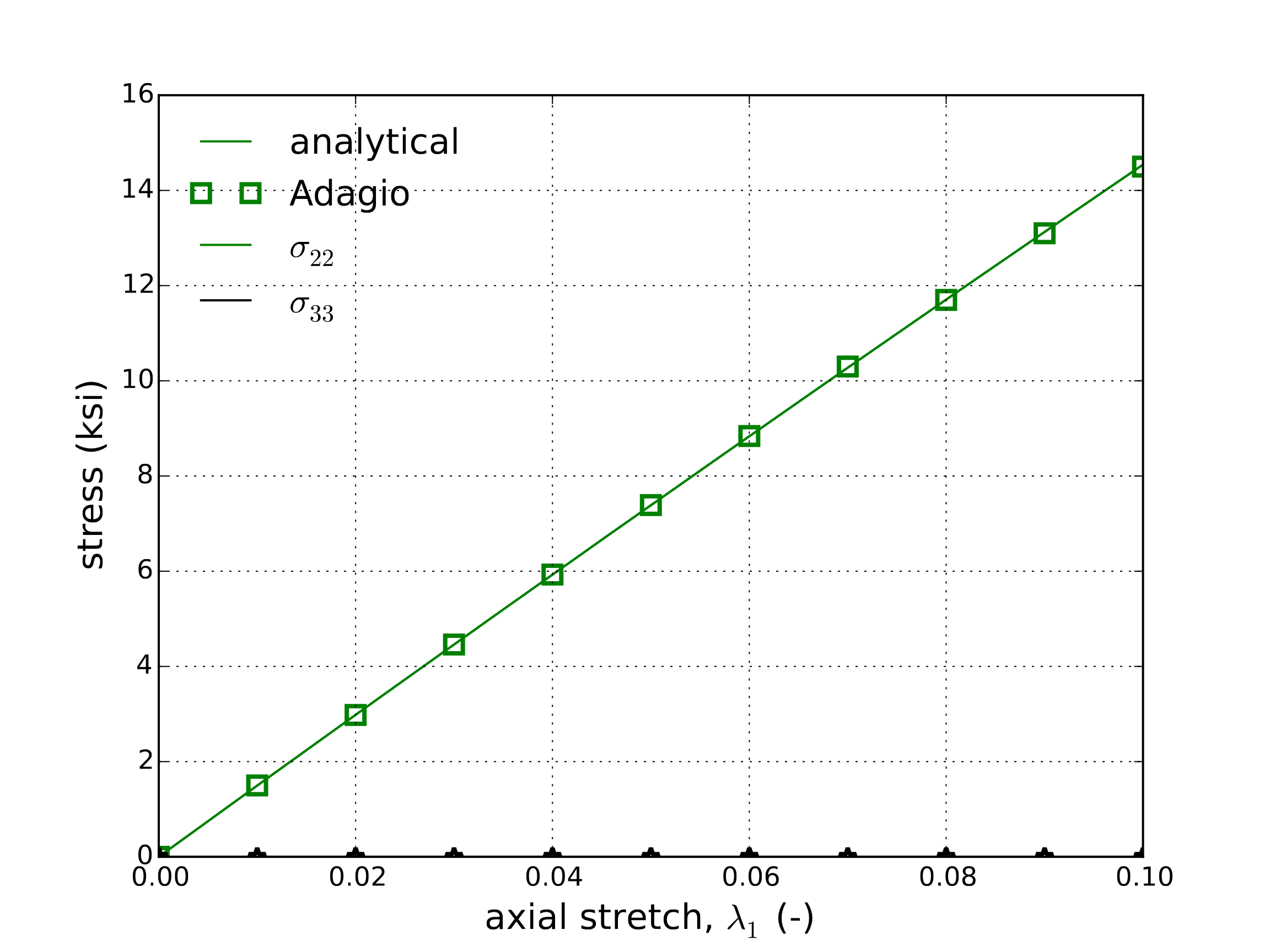
Fig. 4.6 Analytical and numerical results of axial \(\sigma_{11}\) and transverse, \(\sigma_{22}\) and \(\sigma_{33}\), as a function of the stretch \(\lambda_1\).

4.4.3.2. Uniaxial Strain

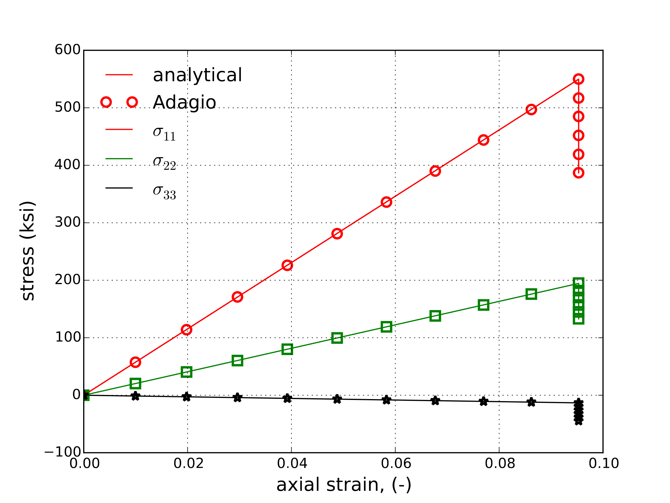
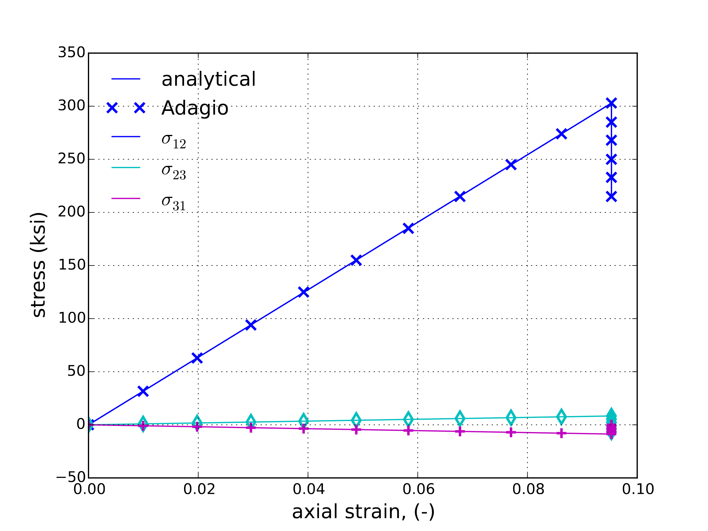
Secondly, the capabilities of this model under arbitrary rotations are explored. To be able to analytically consider this problem, a uniaxial strain (\(\varepsilon_{ij}=\varepsilon_{11}\delta_{i1}\delta_{j1}\)) loading is investigated. The material properties are rotated with the specified orientations per Equations (4.6) and (4.7) using the specified orientations in Table 4.2. A combined thermal-mechanical loading is considered. Specifically, the material is first stretched to the specified strain and that strain is then held fixed during a heating step (\(\Delta T=\)400 K) to investigate the ability of the model to accurately incorporate anisotropic coefficients of thermal expansion. The results for both the analytical and numerical (from a corresponding single element simulation) analyses are shown in Fig. 4.7 with the normal and shear stresses presented in Fig. 4.7(a) and Fig. 4.7(b) respectively. Clear agreement may be seen during both the thermal and mechanical loading stages including the anisotropic effects further verifying model capabilities.

Table 4.2 The coordinate system rotations used with the elastic 3D orthotropic model for the uniaxial strain test.

\(\alpha_1\)	30	Direction 1	3
\(\alpha_2\)	60	Direction 2	1

Normal stresses

Shear stresses

Fig. 4.7 Analytical and numerical results of the stress state through a thermomechanical uniaxial strain loading as a function of the axial strain \(\varepsilon_{11}\).

4.4.4. User Guide

BEGIN PARAMETERS FOR MODEL ELASTIC_3D_ORTHOTROPIC
  #
  # Elastic constants
  #
  YOUNGS MODULUS = <real>
  POISSONS RATIO = <real>
  SHEAR MODULUS  = <real>
  BULK MODULUS   = <real>
  LAMBDA         = <real>
  TWO MU         = <real>
  #
  # Material coordinates system definition
  #
  COORDINATE SYSTEM             = <string> coordinate_system_name
  DIRECTION FOR ROTATION        = <real>   1|2|3
  ALPHA                         = <real>   (degrees)
  SECOND DIRECTION FOR ROTATION = <real>   1|2|3
  SECOND ALPHA                  = <real>   (degrees)
  #
  # Required parameters
  #
  YOUNGS MODULUS AA = <real>
  YOUNGS MODULUS BB = <real>
  YOUNGS MODULUS CC = <real>
  POISSONS RATIO AB = <real>
  POISSONS RATIO BC = <real>
  POISSONS RATIO CA = <real>
  SHEAR MODULUS AB  = <real>
  SHEAR MODULUS BC  = <real>
  SHEAR MODULUS CA  = <real>
  #
  # Thermal strain functions
  #
  THERMAL STRAIN AA FUNCTION = <string>
  THERMAL STRAIN BB FUNCTION = <string>
  THERMAL STRAIN CC FUNCTION = <string>
  #
END [PARAMETERS FOR MODEL ELASTIC_3D_ORTHOTROPIC]

In the above command blocks all of the following are required inputs.

• Even though they are not used within the material model itself, elastic constants are still required input for hourglass control, certain preconditioners, and other various capabilities. After examining various test problems, it has been determined that using the mean of the orthotropic properties as the isotropic elastic constants yields the best results.

• The Young’s moduli corresponding to the principal material axes A, B, and C are given by the YOUNGS MODULUS AA, YOUNGS MODULUS BB, and YOUNGS MODULUS CC command lines.

• The Poisson’s ratio defining the BB normal strain when the material is subjected only to AA normal stress is given by the POISSONS RATIO AB command line.

• The Poisson’s ratio defining the CC normal strain when the material is subjected only to BB normal stress is given by the POISSONS RATIO BC command line.

• The Poisson’s ratio defining the AA normal strain when the material is subjected only to CC normal stress is given by the POISSONS RATIO CA command line.

• The remaining Poisson’s ratios needed for the orthotropic elastic relations (i.e. the BA, CB, and AC Poisson’s ratios) are calculated internally. They are calculated as usual from the given Poisson’s ratios, given Young’s moduli, and energy considerations, which provide expressions for these parameters from the resulting symmetry of the compliance tensor.

• The shear moduli for shear in the AB, BC, and CA planes are given by the SHEAR MODULUS AB, SHEAR MODULUS BC, and SHEAR MODULUS CA command lines, respectively.

• The thermal strain functions for normal thermal strains along the principal material directions are given by the THERMAL STRAIN AA FUNCTION, THERMAL STRAIN BB FUNCTION, and THERMAL STRAIN CC FUNCTION command lines.

Warning

The ELASTIC_3D_ORTHOTROPIC model cannot currently be used in conjunction with the control stiffness implicit solver block.

There are no output variables available for the Elastic Three-Dimensional Orthotropic material model.

---

[1]

A.E. Green and W. Zerna. Theoretical Elasticity, 2nd Edition. Clarendon Press, Oxford, 1968.