4.13. J₂ Plasticity Model

4.13.1. Theory

The \(J_2\) plasticity model is a generic implementation of a von Mises yield surface with kinematic and isotropic hardening features. Unlike other models (e.g. Elastic-Plastic, Elastic-Plastic Power Law) more flexible, general hardening forms are implemented enabling different isotropic hardening descriptions and some rate and/or temperature dependence.

As is common to other plasticity models in LAMÉ, the \(J_2\) plasticity model uses a hypoelastic formulation. As such, the total rate of deformation is additively decomposed into an elastic and plastic part such that

\[D_{ij}=D^{\text{e}}_{ij}+D^{\text{p}}_{ij}.\]

The objective stress rate, depending only on the elastic deformation, may then be written as,

\[\stackrel{\circ}{\sigma}_{ij}=\mathbb{C}_{ijkl}D^{\text{e}}_{kl},\]

where \(\mathbb{C}_{ijkl}\) is the fourth-order elastic, isotropic stiffness tensor.

The yield surface for the \(J_2\) plasticity model, \(f\), may be written,

(4.44)\[f\left(\sigma_{ij},\alpha_{ij},\bar{\varepsilon}^p,\dot{\bar{\varepsilon}}^p,\theta\right)=\phi\left(\sigma_{ij},\alpha_{ij}\right)-\bar{\sigma}\left(\bar{\varepsilon}^p,\dot{\bar{\varepsilon}}^p,\theta\right),\]

in which \(\alpha_{ij},\bar{\varepsilon}^p,\dot{\bar{\varepsilon}}^p,\) and \(\theta\) are the kinematic backstress, equivalent plastic strain, equivalent plastic strain rate, and absolute temperature, respectively, while \(\phi\) and \(\bar{\sigma}\) are the effective stress and a generic form of the flow stress. Broadly speaking, the effective stress describes the shape of the yield surface and kinematic effects while the flow stress gives the size of the current yield surface. It should also be noted that in writing the yield surface in this way, the dependence on the state variables is split between the effective stress and flow stress functions.

For \(J_2\) plasticity, the effective stress is given as,

\[\phi^2\left(\sigma_{ij},\alpha_{ij}\right)=\frac{3}{2}\left(s_{ij}-\alpha_{ij}\right)\left(s_{ij}-\alpha_{ij}\right),\]

with \(s_{ij}\) being the deviatoric stress defined as \(s_{ij}=\sigma_{ij}-(1/3)\sigma_{kk}\delta_{ij}\). For the flow stress, a general representation of the form,

\[\bar{\sigma}\left(\bar{\varepsilon}^p,\dot{\bar{\varepsilon}}^p,\theta\right)=\sigma_y\hat{\sigma}_{\text{y}}\left(\dot{\bar{\varepsilon}}^p\right)\breve{\sigma}_{\text{y}}\left(\theta\right)+K\left(\bar{\varepsilon}^p\right)\hat{\sigma}_{\text{h}}\left(\dot{\bar{\varepsilon}}^p\right)\breve{\sigma}_{\text{h}}\left(\theta\right),\]

is allowed. In this fashion, the effects of rate (\(\hat{\sigma}_{\text{y,h}}\)) and temperature (\(\breve{\sigma}_{\text{y,h}}\)) dependence on yield (\(\sigma_y\)) and isotropic hardening (\(K\left(\bar{\varepsilon}^p\right)\)) are decomposed. Separate temperature and rate dependencies may be be specified for yield (subscript y) and hardening (h). This assumption is an extension of the multiplicative decomposition of the Johnson-Cook model [[1], [2]]. It should be noted that not all effects need to be included and the default parameterization of the hardening classes is such that the response is rate and temperature independent. The following section on plastic hardening will go into more detail on possible choices for functional representations.

An associated flow rule is utilized such that the plastic rate of deformation is normal to the yield surface and is given by,

\[D_{ij}^{\text{p}}=\dot{\gamma}\frac{\partial\phi}{\partial\sigma_{ij}}=\dot{\gamma}\frac{3}{2\phi}s_{ij},\]

where \(\dot{\gamma}\) is the consistency multiplier enforcing \(f=0\) during plastic deformation. Given the form of \(f\), it can also be shown that \(\dot{\gamma}=\dot{\bar{\varepsilon}}^p\).

Additional discussion on options for failure models and adiabatic heating may be found in [[3], [4]] and [[5]], respectively.

4.13.1.1. Plastic Hardening

Plastic hardening refers to increases in the flow stress, \(\bar{\sigma}\), with plastic deformation. As such, hardening is described via a functional relationship between the flow stress and isotropic hardening variable (effective plastic strain), \(\bar{\sigma}\left(\bar{\varepsilon}^p\right)\). Over the course of nearly a century of work in metal plasticity, a variety of relationships have been proposed to describe the interactions associated with different physical interpretations, deformation mechanisms, and materials. To enable the utilization of the same plasticity models for different material systems, a modular implementation of plastic hardening has been adopted such that the analyst may select different hardening models from the input deck thereby avoiding any code changes or user subroutines. In this section, additional details are given for the different models to enable the user to select the appropriate choice of model. Note, the models being discussed here are only for isotropic hardening in which the yield surface expands. Kinematic hardening in which the yield surface translates in stress-space with deformation and distortional hardening where the shape of the yield surface changes shape with deformation are not treated. For a larger discussion of the phenomenology and history of different hardening types, the reader is referred to [[6], [7], [8]].

Given the ubiquitous nature of these hardening laws in computational plasticity, some (if not most) of this material may be found elsewhere in this manual. Nonetheless, the discussion is repeated here for the convenience of the reader.

4.13.1.1.1. Linear

Linear hardening is conceptually the simplest model available in LAMÉ. As the name implies, a linear relationship is assumed between the hardening variable, \(\bar{\varepsilon}^p\), and flow stress. The hardening modulus, \(H^{\prime}\), is a constant giving the rate of change of flow stress with plastic flow. The flow stress expression may therefore be written,

\[\bar{\sigma}=\sigma_y + H^{\prime}\bar{\varepsilon}^p.\]

The simplicity of the model is its main feature as the constant slope,

\[\frac{d\bar{\sigma}}{d\bar{\varepsilon}^p}=H^{\prime},\]

makes the model attractive for analytical models and cheap for computational implementations (e.g. radial return algorithms require only a single correction step). Unfortunately, the simplicity of the representation also means that it has limited predictive capabilities and can lead to overly stiff responses.

4.13.1.1.2. Power Law

Another common expression for isotropic hardening is the power-law hardening model. Due to its prevalence, a dedicated ELASTIC-PLASTIC POWER LAW HARDENING model may be found in LAMÉ (see Section 4.8.1). This expression is given as,

\[\bar{\sigma}=\sigma_y + A<\bar{\varepsilon}^p-\varepsilon_L>^n,\]

in which \(<\cdot>\) are Macaulay brackets, \(\varepsilon_L\) is the Luders strain, \(A\) is a fitting constant, and \(n\) is an exponent typically taken such that \(0<n\leq1\). The Luders strain is a positive, constant strain value (defaulted to zero) giving an initially perfectly plastic response in the plastic deformation domain (see Fig. 4.20). The derivative is then simply,

\[\frac{d\bar{\sigma}}{d\bar{\varepsilon}^p}=nA<\bar{\varepsilon}^p-\varepsilon_L>^{\left(n-1\right)}.\]

Note, one difficulty in such an implementation is that when the effective equivalent plastic strain is zero, numerical difficulties may arise in evaluating the derivative and necessitate special treatment of the case.

4.13.1.1.3. Voce

The Voce hardening model (sometimes referred to as a saturation model) uses a decaying exponential function of the equivalent plastic strain such that the hardening eventually saturates to a specified value (thus the name). Such a relationship has been observed in some structural metals giving rise to the popularity of the model. The hardening response is given as,

\[\bar{\sigma}=\sigma_y + A\left(1-\exp\left(-n\bar{\varepsilon}^p\right)\right),\]

in which \(A\) is a fitting constant and \(n\) is a fitting exponent controlling how quickly the hardening saturates. Importantly, the derivative is written as,

\[\frac{d\bar{\sigma}}{d\bar{\varepsilon}^p}=nA\exp\left(-n\bar{\varepsilon}^p\right),\]

and is well defined everywhere giving the selected form an advantage over the aforementioned power law model.

4.13.1.1.4. Johnson-Cook

The Johnson-Cook hardening model is a variant of the classical Johnson-Cook [[1], [2]] expression. In this instance, the temperature-dependence is neglected to focus on the rate-dependent capabilities while allowing for arbitrary isotropic hardening forms via the use of a user-defined hardening function. With these assumptions, the flow stress may be written as,

\[\bar{\sigma}=\tilde{\sigma}_y\left(\bar{\varepsilon}^p\right)\left[1+C\left<\ln\left(\frac{\dot{\bar{\varepsilon}}^p}{\dot{\varepsilon}_0}\right)\right>\right],\]

in which \(\tilde{\sigma}_y\left(\bar{\varepsilon}^p\right)\) is the user-specified rate-independent hardening function, \(C\) is a fitting constant and \(\dot{\varepsilon}_0\) is a reference strain rate. The Macaulay brackets ensure the material behaves in a rate independent fashion when \(\dot{\bar{\varepsilon}}^p < \dot{\varepsilon}_0\).

4.13.1.1.5. Power Law Breakdown

Like the Johnson-Cook formulation, the power-law breakdown model is also rate-dependent. Again, a multiplicative decomposition is assumed between isotropic hardening and the corresponding rate-dependence dependent. In this case, however, the functional form is derived from the analysis of Frost and Ashby [[9]] in which power-law relationships like those of the Johnson-Cook model cease to appropriately capture the physical response. The form used here is similar to the expression used by Brown and Bammann [[10]] and is written as,

\[\bar{\sigma} = \tilde{\sigma}_y\left(\bar{\varepsilon}^p\right)\left[1+\text{asinh}\left(\left(\frac{\dot{\bar{\varepsilon}}^p}{g}\right)^{\left(1/m\right)}\right)\right],\]

with \(\tilde{\sigma}_y\left(\bar{\varepsilon}^p\right)\) being the user supplied rate independent expression, \(g\) is a model parameter related to the activation energy required to transition from climb to glide-controlled deformation, and \(m\) dictates the strength of the dependence.

4.13.1.2. Flow Stress

Unlike the previously described models, the flow-stress hardening method is less a specific physical representation and more a generalization of hardening behaviors to allow greater flexibility in separately describing isotropic hardening, rate-dependence, and temperature dependence. As such, the generic flow-stress definition of

\[\bar{\sigma}\left(\bar{\varepsilon}^p,\dot{\bar{\varepsilon}}^p,\theta\right)=\tilde{\sigma}_y\left(\bar{\varepsilon}^p\right)\hat{\sigma}\left(\dot{\bar{\varepsilon}}^p\right)\breve{\sigma}\left(\theta\right),\]

is used in which \(\hat{\sigma}\) and \(\breve{\sigma}\) are rate and temperature multipliers, respectively, that by default are unity (such that the response is rate and temperature independent). The isotropic hardening component, \(\tilde{\sigma}_y\), is specified as,

\[\tilde{\sigma}_y=\sigma_y+K\left(\bar{\varepsilon}^p\right),\]

with \(\sigma_y\) being the constant yield stress and \(K\) is the isotropic hardening that is initially zero and a function of the equivalent plastic strain. A multiplicative decomposition such as this mirrors the general structure used by Johnson and Cook [[1], [2]] although greater flexibility is allowed in terms of the specific form of the rate and temperature multipliers.

Given the aforementioned defaults for rate and temperature dependence, the corresponding multipliers need not be specified. A representation for the isotropic hardening, however, must be specified and can be defined via linear, power-law, Voce, or user-defined representations. For the user-defined case, an isotropic hardening function is required and it must be highlighted that the interpretation differs from the general user-defined hardening model. In this case, as the specified function represents the isotropic hardening, it should start from zero – not yield.

Although the flow-stress hardening model defaults to rate and temperature independent, a multiplier may be defined for either (or both) of the terms. For rate-dependence, either the previously discussed Johnson-Cook or power-law breakdown models or a user-defined multiplier may be used. For the user-defined capability, the multiplier should be input as a strictly positive function of the equivalent plastic strain rate with a value of one in the rate-independent limit.

In terms of temperature dependence, the multiplier may be specified given a Johnson-Cook dependency [[1], [2]],

\[\breve{\sigma}\left(\theta\right)=1-\left(\frac{\theta-\theta_{\text{ref}}}{\theta_{\text{melt}}-\theta_{\text{ref}}}\right)^M,\]

with \(\theta_{\text{ref}},~\theta_{\text{melt}}\) and \(M\) being the reference temperature, melting temperature, and temperature exponent. The temperature multiplier may also be specified via a user defined function.

4.13.1.3. Decoupled Flow Stress

Like the flow-stress hardening method, the decoupled flow-stress hardening implementation is a generalization of the hardening behaviors to allow greater flexibility. In differentiating the two, for the decoupled model the rate and temperature dependence may be separately specified for the yield and hardening portions of the flow stress. As such, the generic flow-stress definition of

\[\bar{\sigma}\left(\bar{\varepsilon}^p,\dot{\bar{\varepsilon}}^p,\theta\right)=\sigma_y\hat{\sigma}_{\text{y}}\left(\dot{\bar{\varepsilon}}^p\right)\breve{\sigma}_{\text{y}}\left(\theta\right)+K\left(\bar{\varepsilon}^p\right)\hat{\sigma}_{\text{h}}\left(\dot{\bar{\varepsilon}}^p\right)\breve{\sigma}_{\text{h}}\left(\theta\right),\]

is used in which \(\hat{\sigma}\) and \(\breve{\sigma}\) are rate and temperature multipliers, respectively, that by default are unity (such that the response is rate and temperature independent) with subscripts y and h denoting functions associated with yield and hardening. The isotropic hardening is described by \(K\left(\bar{\varepsilon}^p\right)\) and \(\sigma_y\) is the constant initial yield stress. It may also be seen that if the yield and hardening dependencies are the same (\(\hat{\sigma}_{\text{y}}=\hat{\sigma}_{\text{h}}\) and \(\breve{\sigma}_{\text{y}}=\breve{\sigma}_{\text{h}}\)) the decoupled flow stress model reduces to that of the flow stress case and mirrors the general structure of the Johnson-Cook model [[1], [2]].

Given the aforementioned defaults for rate and temperature dependence, the corresponding multipliers need not be specified. A representation for the isotropic hardening, however, must be specified and can be defined via linear, power-law, Voce, or user-defined representations. For the user-defined case, an isotropic hardening function should be used and it must be highlighted that the interpretation differs from the general user-defined hardening model. In this case, as the specified function represents the isotropic hardening, it should start from zero – not yield.

Although the decoupled flow-stress hardening model defaults to rate and temperature independent, a multiplier may be defined for any of the terms. For rate-dependence, either the previously discussed Johnson-Cook or power-law breakdown models or a user-defined multiplier may be used. For the user-defined capability, the multiplier should be input as a strictly positive function of the equivalent plastic strain rate with a value of one in the rate-independent limit.

In terms of temperature dependence, the multiplier may be specified given a Johnson-Cook dependency [[1], [2]],

\[\breve{\sigma}\left(\theta\right)=1-\left(\frac{\theta-\theta_{\text{ref}}}{\theta_{\text{melt}}-\theta_{\text{ref}}}\right)^M,\]

where \(\theta_{\text{ref}},~\theta_{\text{melt}}\), and \(M\) are the reference temperature, melting temperature, and temperature exponent. A temperature multiplier may also be specified via a user defined function.

4.13.2. Implementation

The \(J_2\) plasticity model is implemented using a radial return predictor-corrector algorithm. First, an elastic trial stress state is calculated. This is done by assuming that the rate of deformation is completely elastic,

\[T^{tr}_{ij} = T^{n}_{ij} + \Delta t \left( \lambda\delta_{ij}d_{kk} + 2\mu d_{ij} \right).\]

The trial stress state is decomposed into a pressure and a deviatoric stress

\[p^{tr} = \frac{1}{3} T^{tr}_{kk} \;\;\; ; \;\;\; s^{tr}_{ij} = T^{tr}_{ij} - p^{tr}\delta_{ij}.\]

A trial yield function value, \(f^{tr}\), is calculated by assuming purely thermoelastic deformations (\(\dot{\bar{\varepsilon}}^p=0, \bar{\varepsilon}^p_{tr}=\bar{\varepsilon}^p_n\)) such that,

\[f^{tr} \left( s^{tr}_{ij},\alpha_{ij}^n,\bar{\varepsilon}^{p}_n,\dot{\bar{\varepsilon}}^p_{tr}=0,\theta_{n+1} \right) = \phi^{tr}\left(s^{tr}_{ij},\alpha_{ij}^n \right) - \bar{\sigma}\left( \bar{\varepsilon}^{p}_n,\dot{\bar{\varepsilon}}^p_{tr}=0,\theta_{n+1} \right).\]

If \(f^{tr} \leq 0\) then the strain rate is elastic and the stress update is finished. If \(f^{tr} > 0\) then plastic deformation has occurred and a radial return algorithm determines the extent of plastic deformation.

The normal to the yield surface is assumed to lie in the direction of the trial stress state. This gives the following expression for \(N_{ij}\),

\[N_{ij} = \frac{\left(s_{ij}^{tr}-\alpha^n_{ij}\right)}{\|\left(s_{ij}^{tr}-\alpha_{ij}^n\right)\|}.\]

Using a backward Euler algorithm, the final deviatoric stress state is

\[s^{n+1}_{ij} = s_{ij}^{tr} - \Delta \, t 2\mu d_{ij}^{\text{p}},\]

where the plastic strain increment is

\[\Delta d_{ij}^{\text{p}} = \sqrt{\frac{3}{2}} \Delta\bar{\varepsilon}^{p} N_{ij}.\]

The equation for the change in the equivalent plastic strain over the load step is found as the solution to

\[3 \mu \Delta\bar{\varepsilon}^{p} + \bar{\sigma}\left( \bar{\varepsilon}_{n} + \Delta\bar{\varepsilon}^{p}, \Delta t, \theta_{n+1} \right) - \phi^{tr} + f_{n} = 0,\]

in which the plastic strain rate is approximated as, \(\dot{\bar{\varepsilon}}^p=\Delta\bar{\varepsilon}^p/\Delta t\).

4.13.3. Verification

The \(J_2\) plasticity model is verified through a series of uniaxial stress and pure shear tests considering a variety of hardening models. Specifically, the boundary value problems of Appendix A are used. Throughout these tests, the elastic properties are maintained as \(E=70\) GPa and \(\nu = 0.25\).

Additional verification exercises for the various failure models and adiabatic heating capabilities may be found in [[3]], [[4]] and [[5]], respectively.

4.13.3.1. Plastic Hardening

For the verification of the \(J_2\) model, a series of tests using different rate independent, rate dependent, and combinations of these hardening models are investigated for both uniaxial stress and pure shear. For these cases, by imposing a constant plastic strain rate as described in Appendix A the model response may be analytically determined as a function of time. For the rate independent cases, a constant rate of \(\dot{\bar{\varepsilon}}^p=1\times10^{-4} \text{s}^{-1}\) is used to replicate quasi-static conditions.

The various rate dependent and rate independent hardening coefficients are found in Table 4.16 while the remaining model parameters are unchanged from the previous verification exercises. For the current verification exercises, the rate independent hardening models (linear, Voce, and power-law) and rate dependent forms (Johnson-Cook, power-law breakdown) are examined.

Table 4.16 The model parameters for the hardening verification tests used with the \(J_2\) plasticity model during verification tests. Parameters for the rate independent hardening functions, \(\tilde{\sigma}_y\), are also given and denoted with a \(\tilde{\cdot}\) while the subscript refers to the functional form.

\(C\)	0.1	\(\dot{\varepsilon}_0\)	\(1\times 10^{-4}\) s\(^{-1}\)
\(g\)	0.21 s\(^{-1}\)	\(m\)	16.4
\(\tilde{H}_{\text{Linear}}\)	200 MPa
\(\tilde{A}_{\text{PL}}\)	400 MPa	\(\tilde{n}_{\text{PL}}\)	0.25
\(\tilde{A}_{\text{Voce}}\)	200 MPa	\(\tilde{n}_{\text{Voce}}\)	20
\(\sigma_y\)	200 MPa

4.13.3.1.1. Rate-Independent

First, the ability of the built-in rate independent hardening models is assessed in both uniaxial stress and pure shear. Specifically, the linear, power-law, and Voce hardening models are considered and the results determined analytically and numerically via Sierra are presented in Fig. 4.37. As expected, excellent agreement is noted between the two sets of results. Importantly, as the responses of all three rate independent isotropic hardening models are presented in the same figures, the corresponding behaviors can be seen. Note, the given parameterizations are not selected for any form of equivalency. Nonetheless, the linear post-yielding behavior of the linear model can be seen and compared to the non-linear responses of the Voce and power-law implementations. The critical difference between the latter two being that the Voce response saturates at a stress level while the power-law continues to grow.

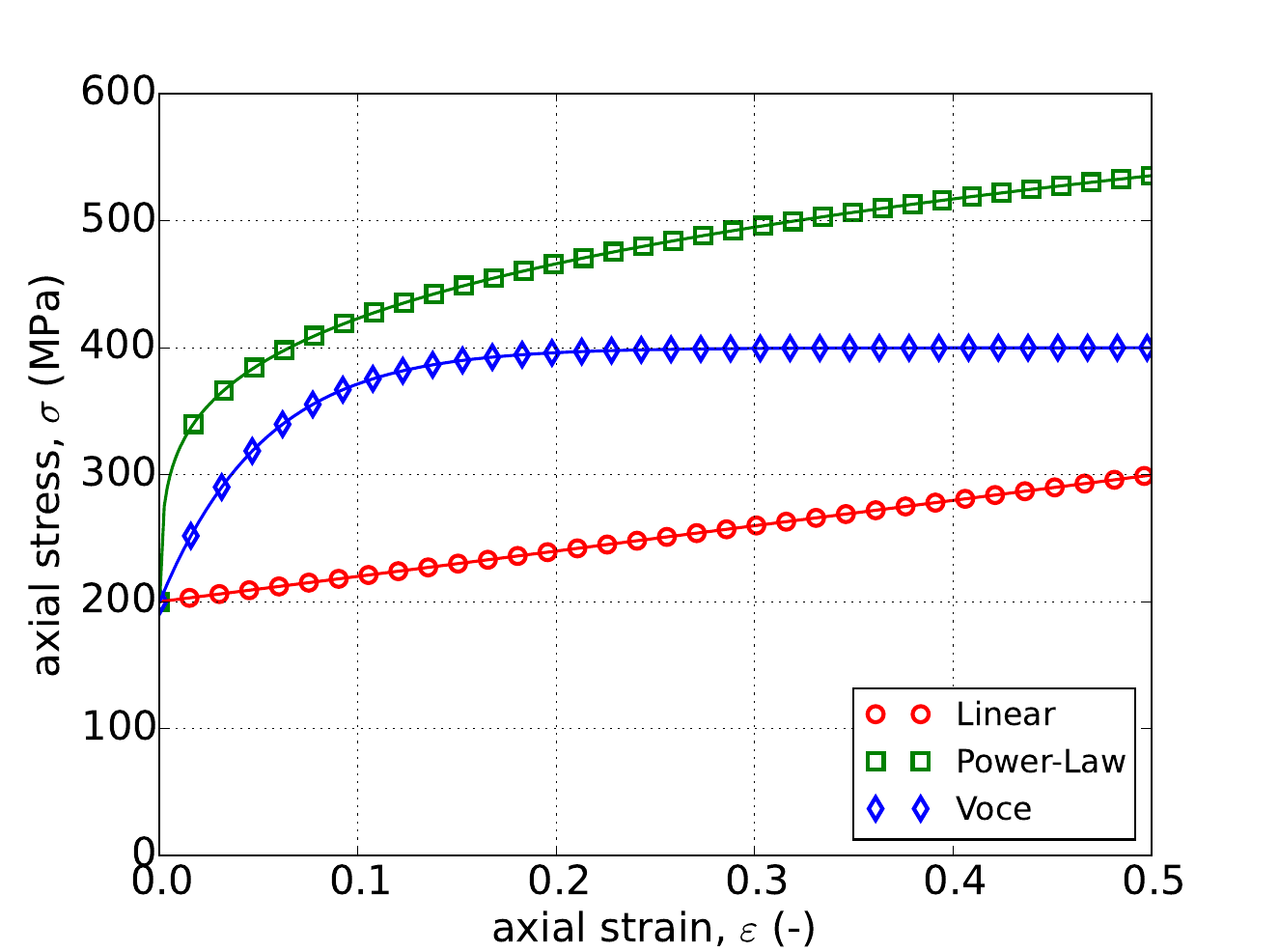Uniaxial Stress

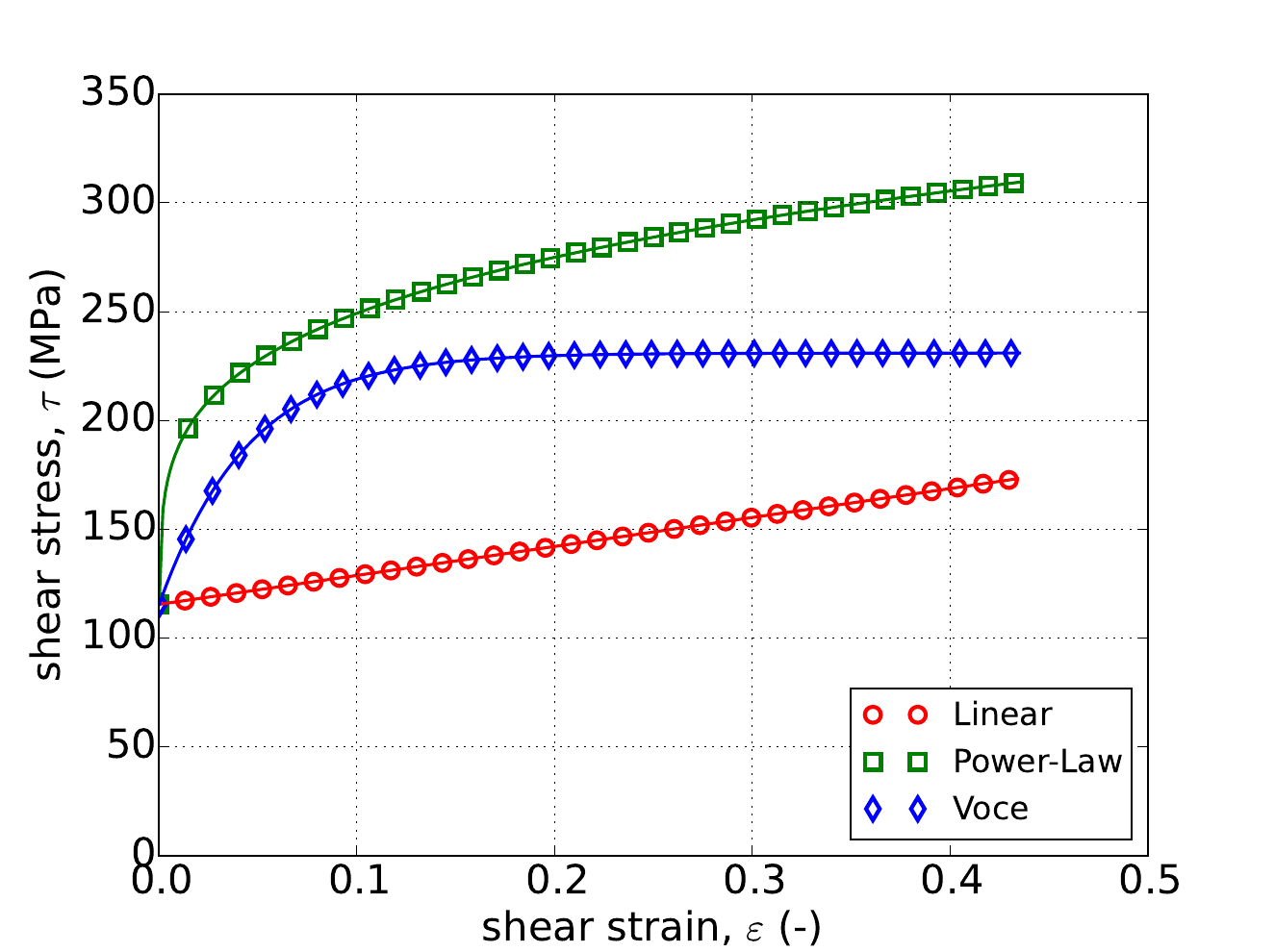Pure Shear

Fig. 4.37 Analytical and numerical (Sierra) (a) uniaxial stress-strain and (b) pure shear responses of the \(J_2\) plasticity model with linear, power-law, and Voce rate independent isotropic hardening. Solid lines are analytical while open symbols are numerical.

4.13.3.1.2. Rate-Dependent

With the performance of the model under rate independent conditions established, next the capabilities of the rate dependent (Johnson-Cook and power-law breakdown) formulations are considered. Note, the flow-stress and decoupled flow-stress models that incorporate more flexible descriptions of isotropic hardening and rate and temperature dependence are left to later sections. With the current Johnson-Cook and power-law breakdown models, user-defined analytic functions are used for each of the specified rate independent hardening functions.

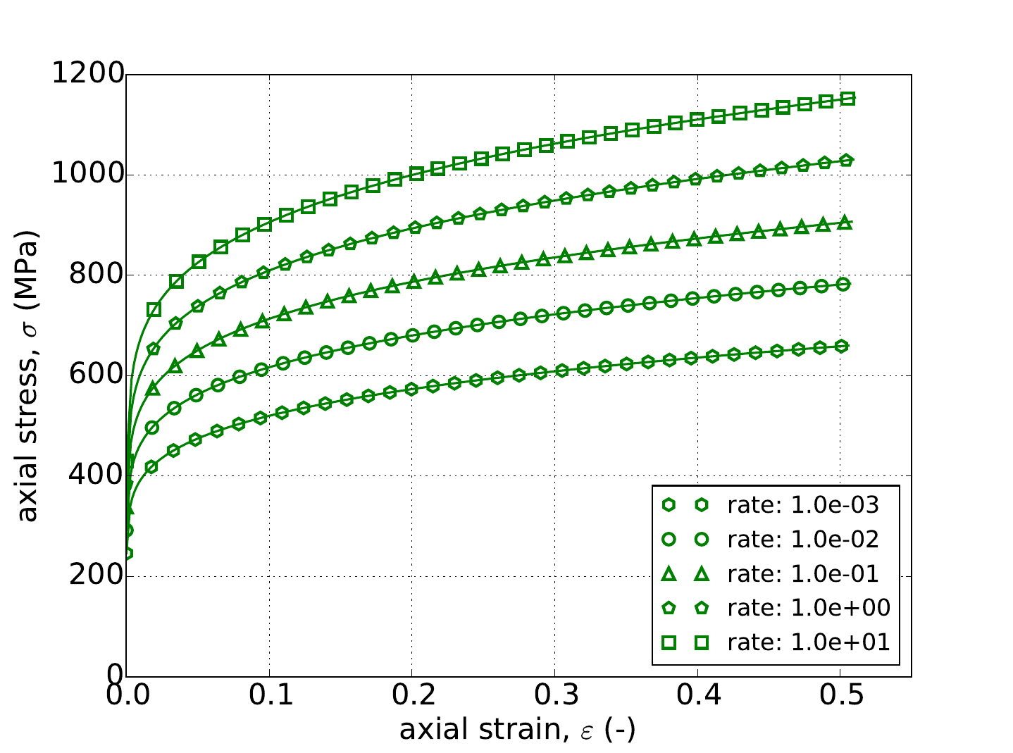
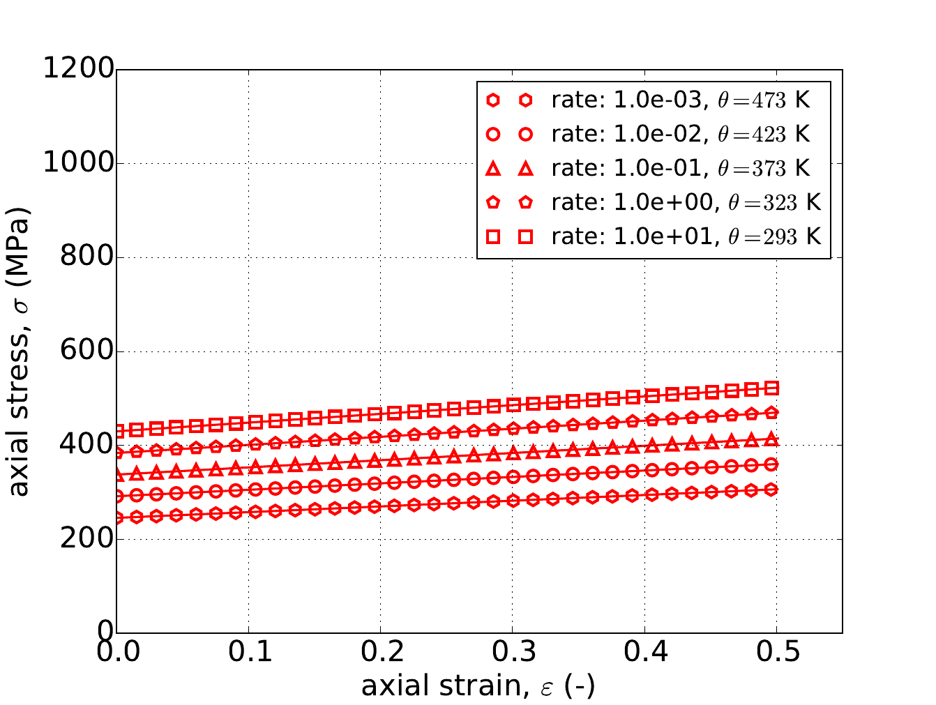
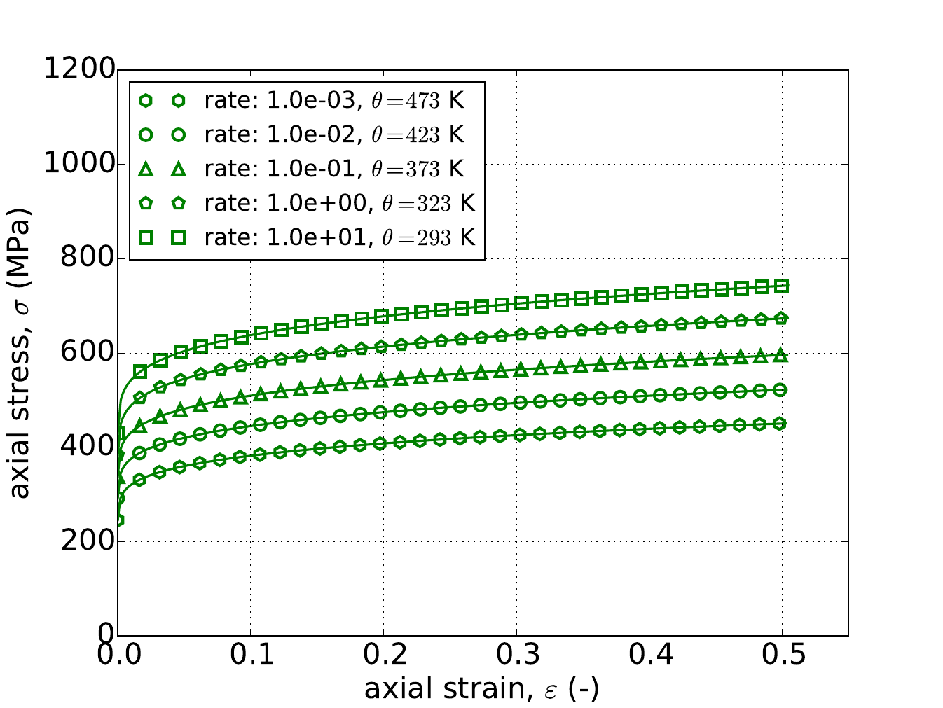
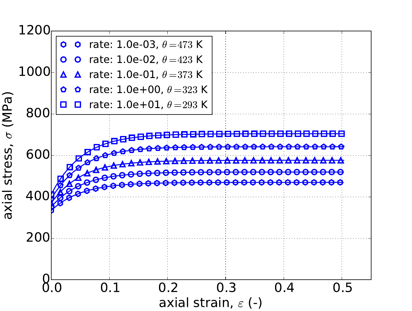
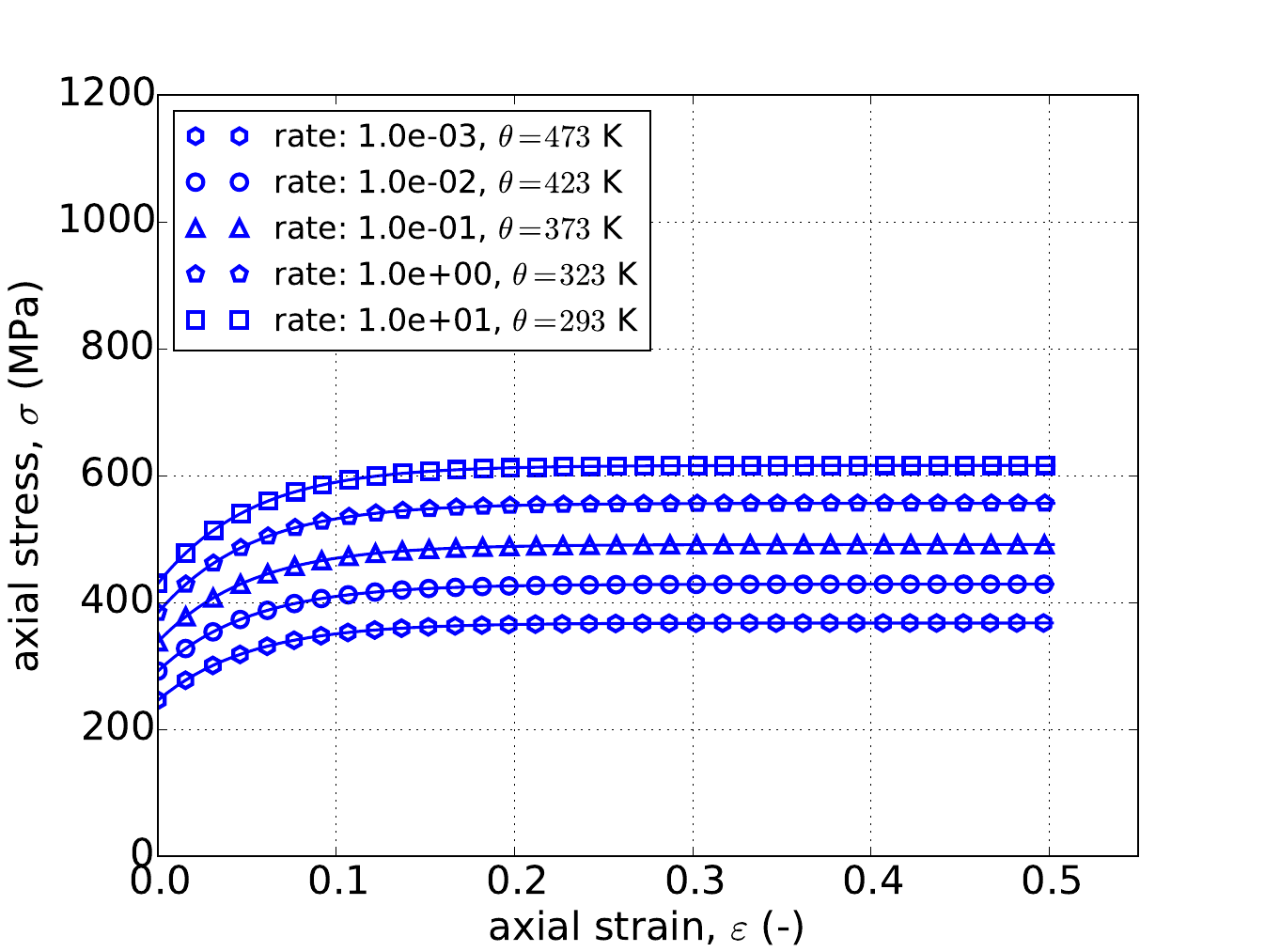
The uniaxial stress-strain responses are interrogated for the Johnson-Cook and power-law breakdown rate dependent hardening models considering linear, power-law, and Voce isotropic hardening in Fig. 4.38. Five decades of plastic strain rates \(\dot{\bar{\varepsilon}}^p=1\times10^{-3}\rightarrow1\times10^{1}\text{s}^{-1}\) are considered. In comparing the analytical and numerical results between all of the cases exceptional agreement is noted between every case.

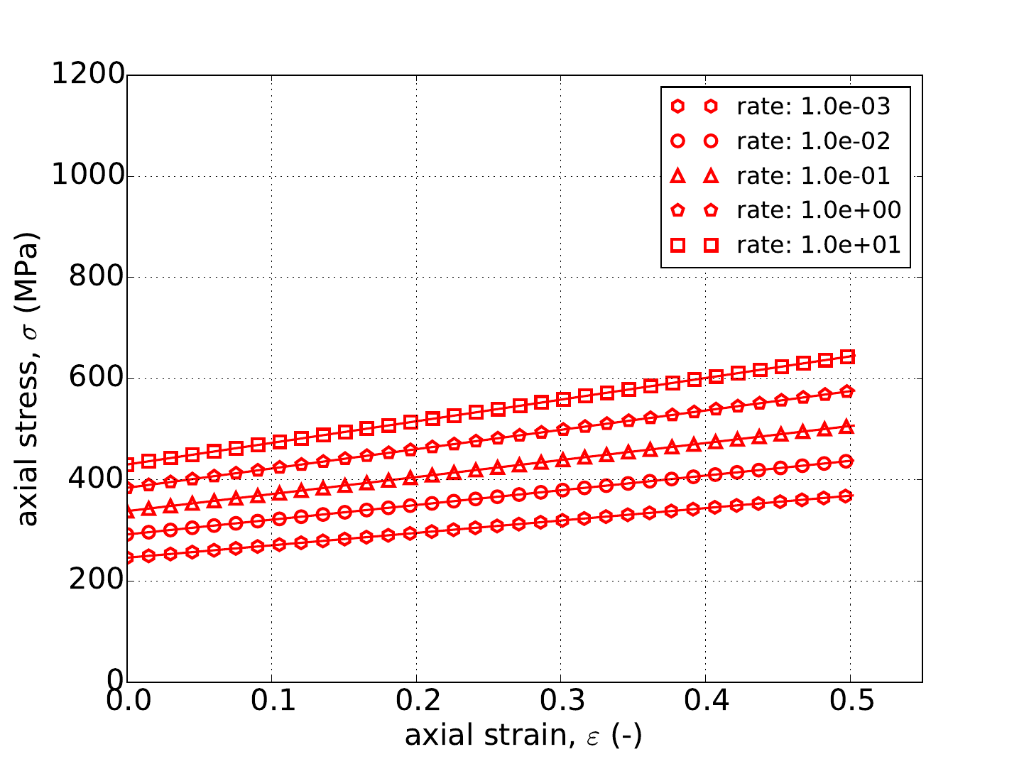Linear, Johnson-Cook

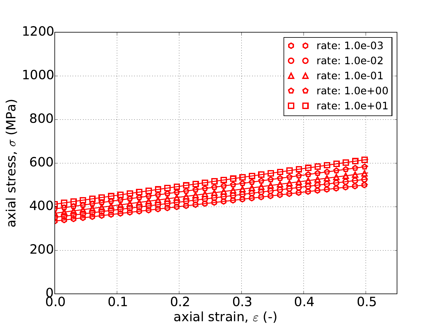Linear, Power-Law Breakdown

Power-Law, Johnson-Cook

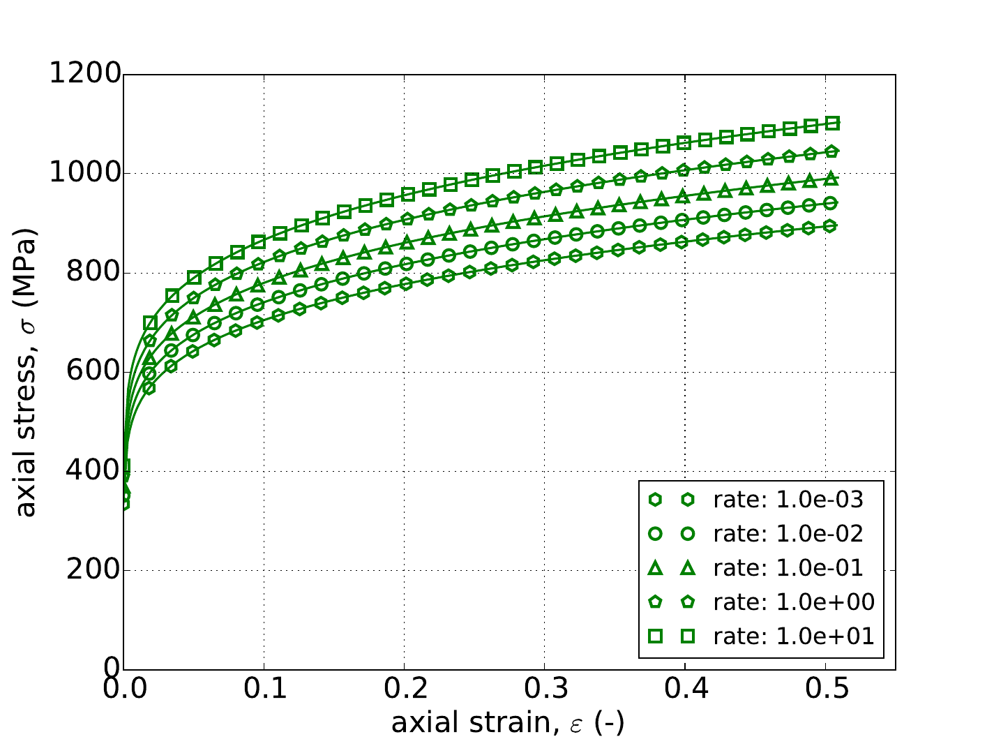Power-Law, Power-Law Breakdown

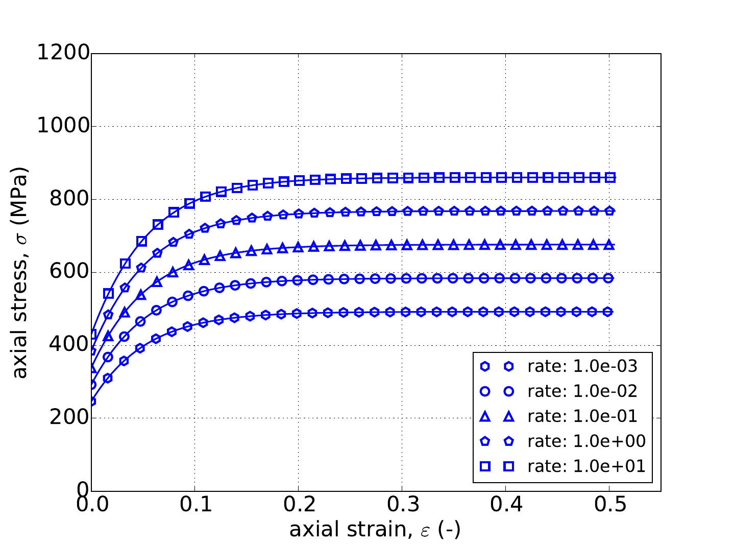Voce, Johnson-Cook

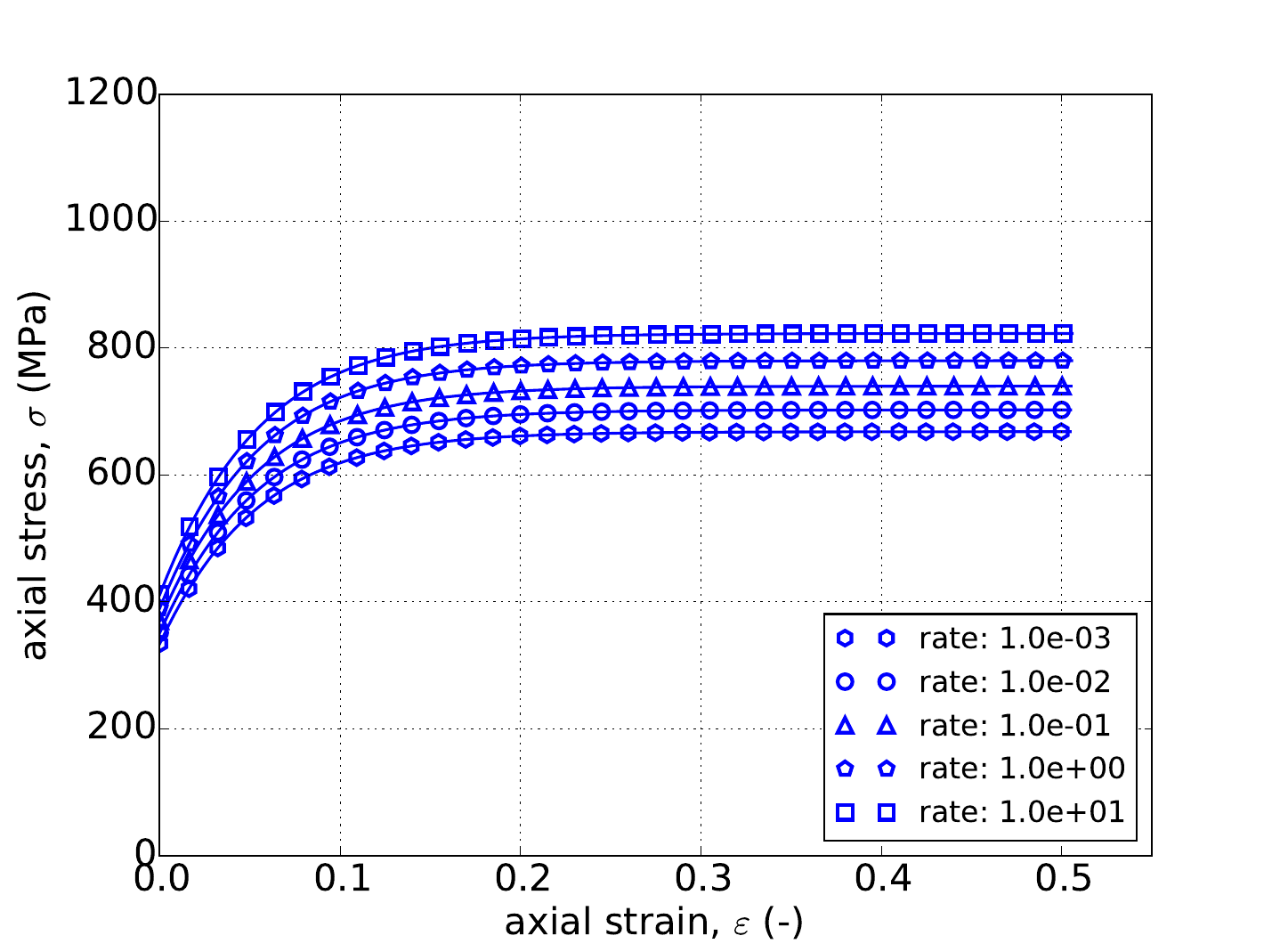Voce, Power-Law Breakdown

Fig. 4.38 Uniaxial stress-strain responses of the \(J_2\) plasticity model with (a,b) linear, (c,d) power-law, and (e,f) Voce isotropic hardening with the (a,c,e) Johnson-Cook and (b,d,f) Power-law breakdown rate dependent hardening models. Solid lines are analytical while open symbols are numerical (Sierra).

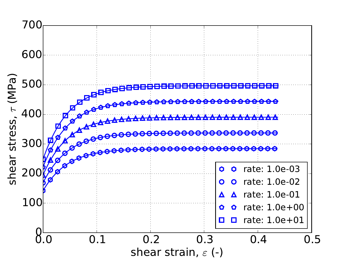
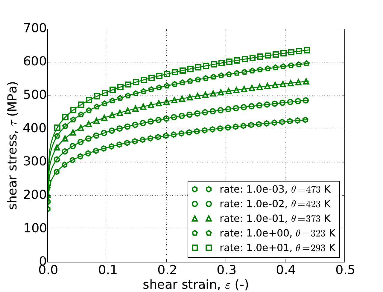
Similarly, the pure shear responses of the six hardening combinations over the five plastic strain rates are given in Fig. 4.39 for both analytical and numerical approaches. As with the normal cases, outstanding agreement is noted between the various results. Thus, between the plethora of problems presented in Fig. 4.38 and Fig. 4.39 the performance of the rate-dependent models may be considered verified.

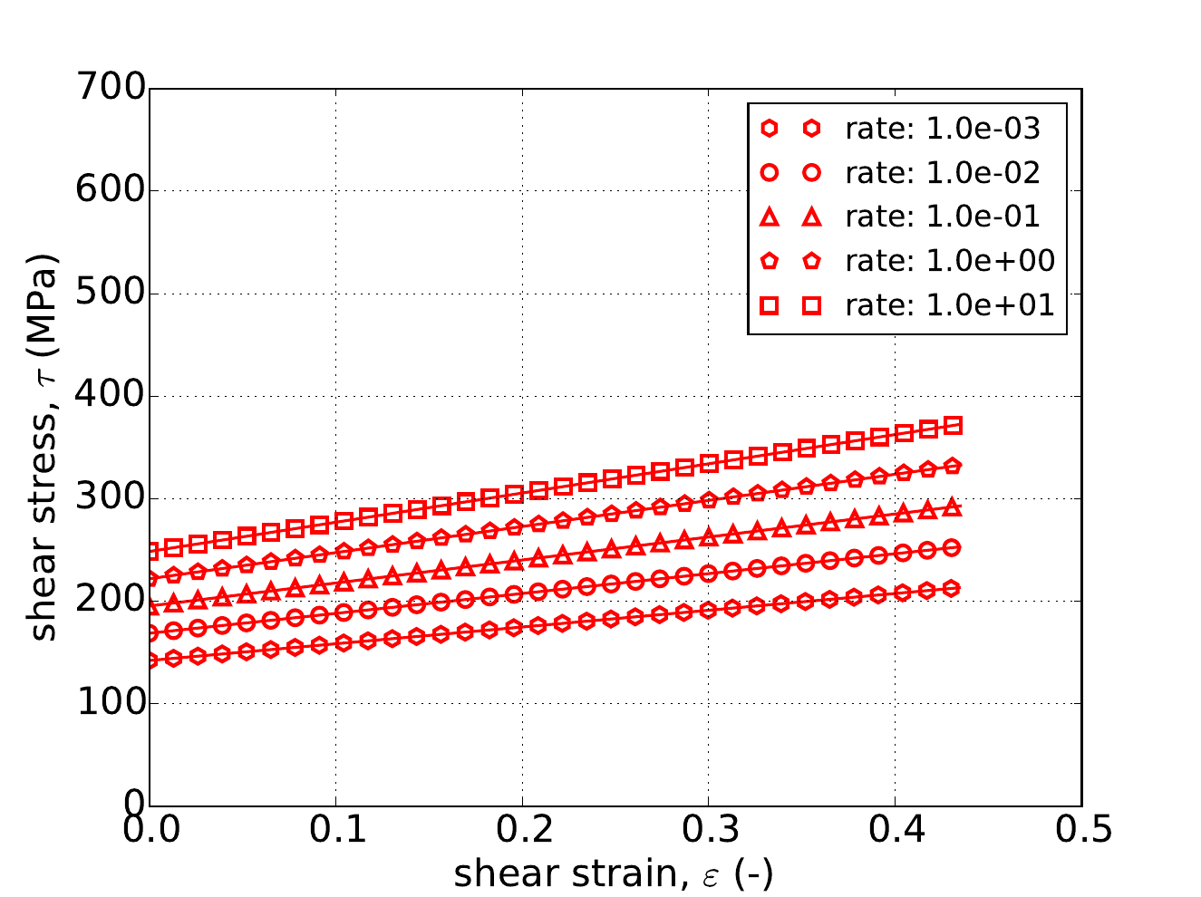Linear, Johnson-Cook

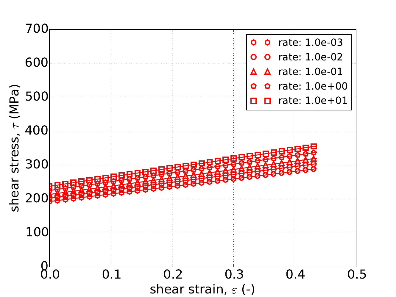Linear, Power-Law Breakdown

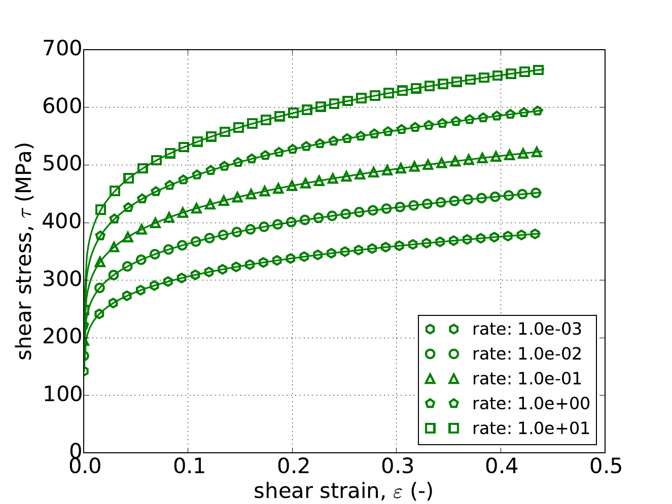Power-Law, Johnson-Cook

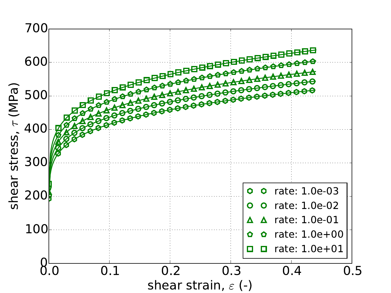Power-Law, Power-Law Breakdown

Voce, Johnson-Cook

Voce, Power-Law Breakdown

Fig. 4.39 Pure shear responses of the \(J_2\) plasticity model with (a,b) linear, (c,d) power-law, and (e,f) Voce isotropic hardening with the (a,c,e) Johnson-Cook and (b,d,f) Power-law breakdown rate dependent hardening models. Solid lines are analytical while open symbols are numerical (Sierra).

4.13.3.1.3. Flow Stress

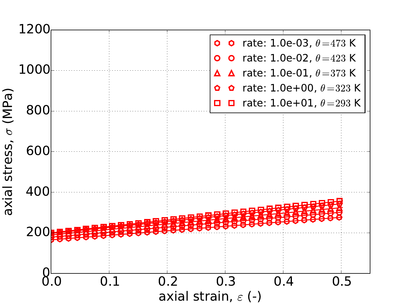
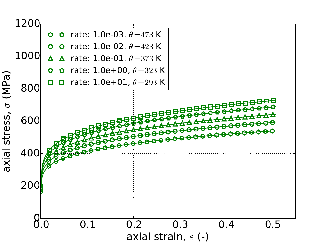
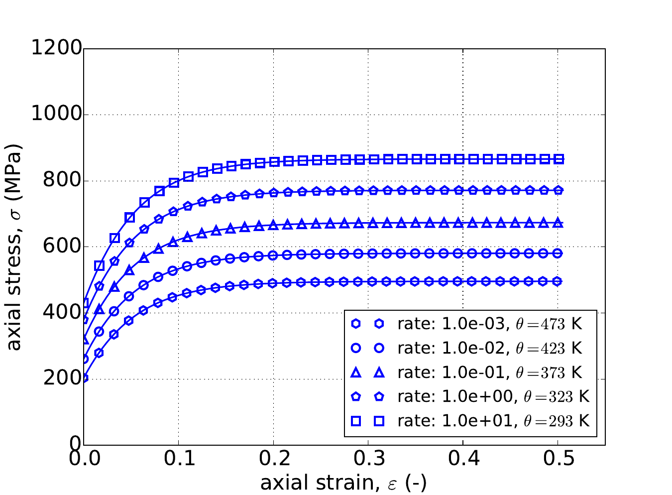
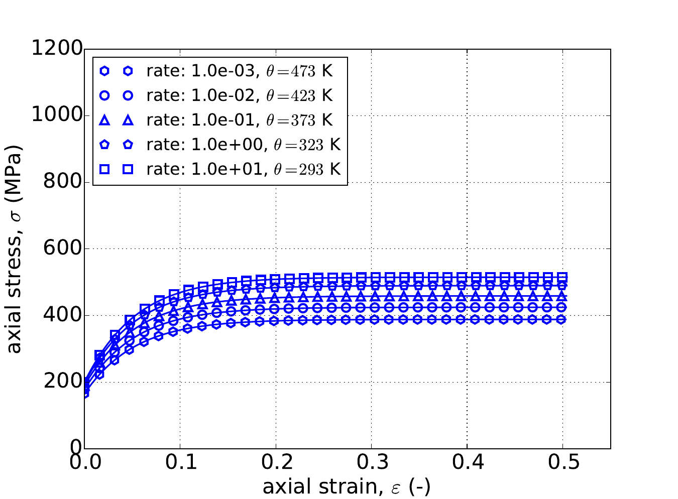
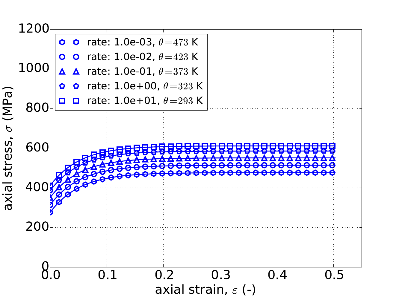
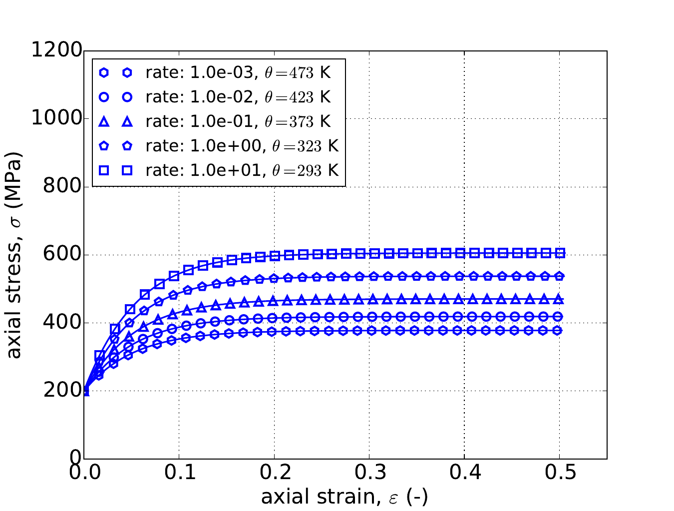
As a next step in verification, the capabilities of the flow-stress hardening model incorporating rate- and temperature-dependence is assessed. To this end, Fig. 4.40 presents uniaxial stress-strain responses considering linear, power-law, and Voce isotropic hardening models with both Johnson-Cook and power-law breakdown rate dependent multipliers and Johnson-Cook type temperature dependence. Five decades of strain rates along with temperatures spanning 180 K are considered in the various figures. In all of the results, agreement is noted between analytical and numerical results.

Linear, Johnson-Cook

Linear, Power-Law Breakdown

Power-Law, Johnson-Cook

Power-Law, Power-Law Breakdown

Voce, Johnson-Cook

Voce, Power-Law Breakdown

Fig. 4.40 Uniaxial stress-strain responses of the \(J_2\) plasticity model using the flow-stress hardening model comprised of (a,b) linear, (c,d) power-law, and (e,f) Voce isotropic hardening, (a,c,e) Johnson-Cook and (b,d,f) power-law breakdown rate multipliers, and (a-f) Johnson-Cook temperature multipliers. Solid lines are analytical while open symbols are numerical (Sierra).

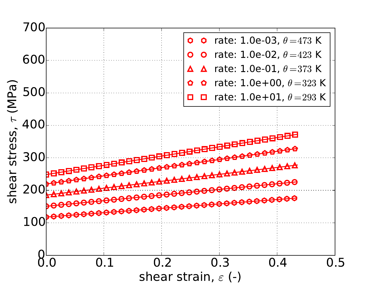
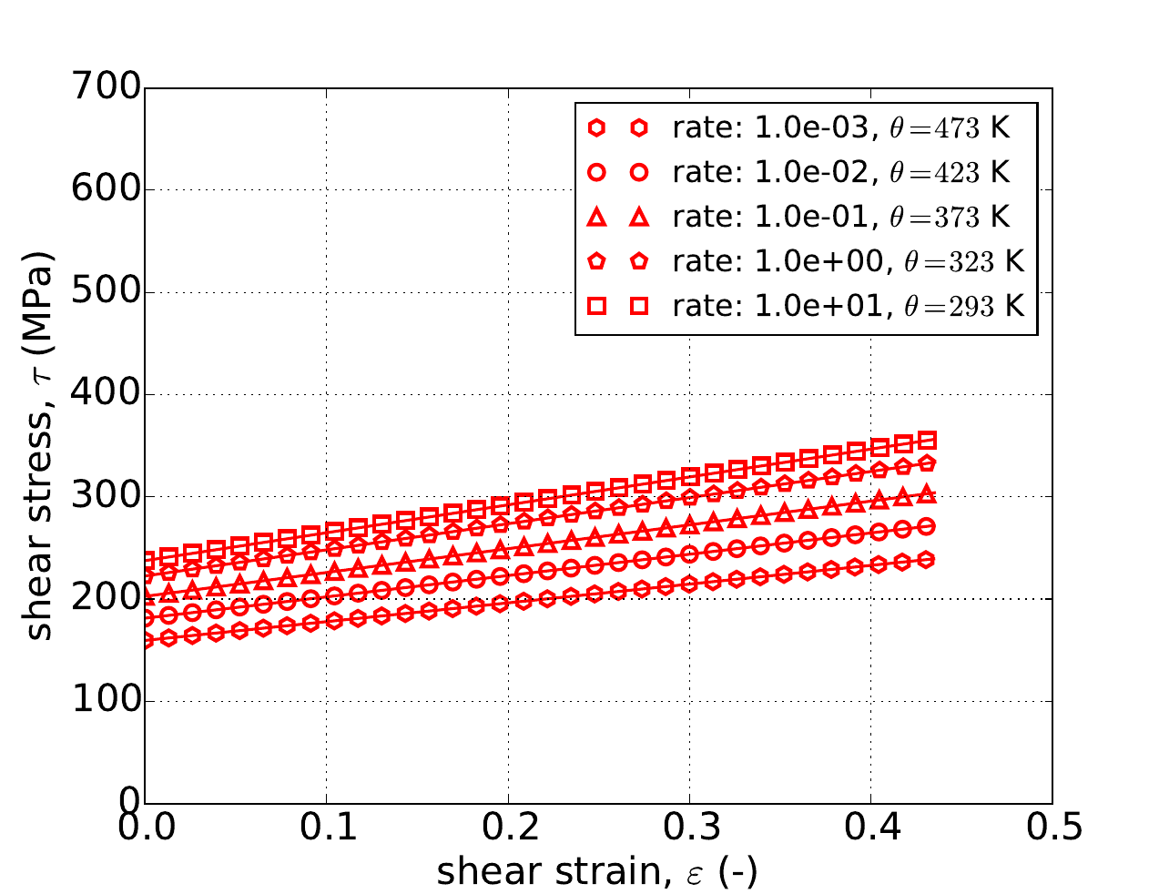
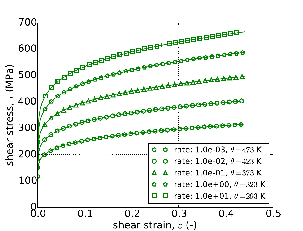
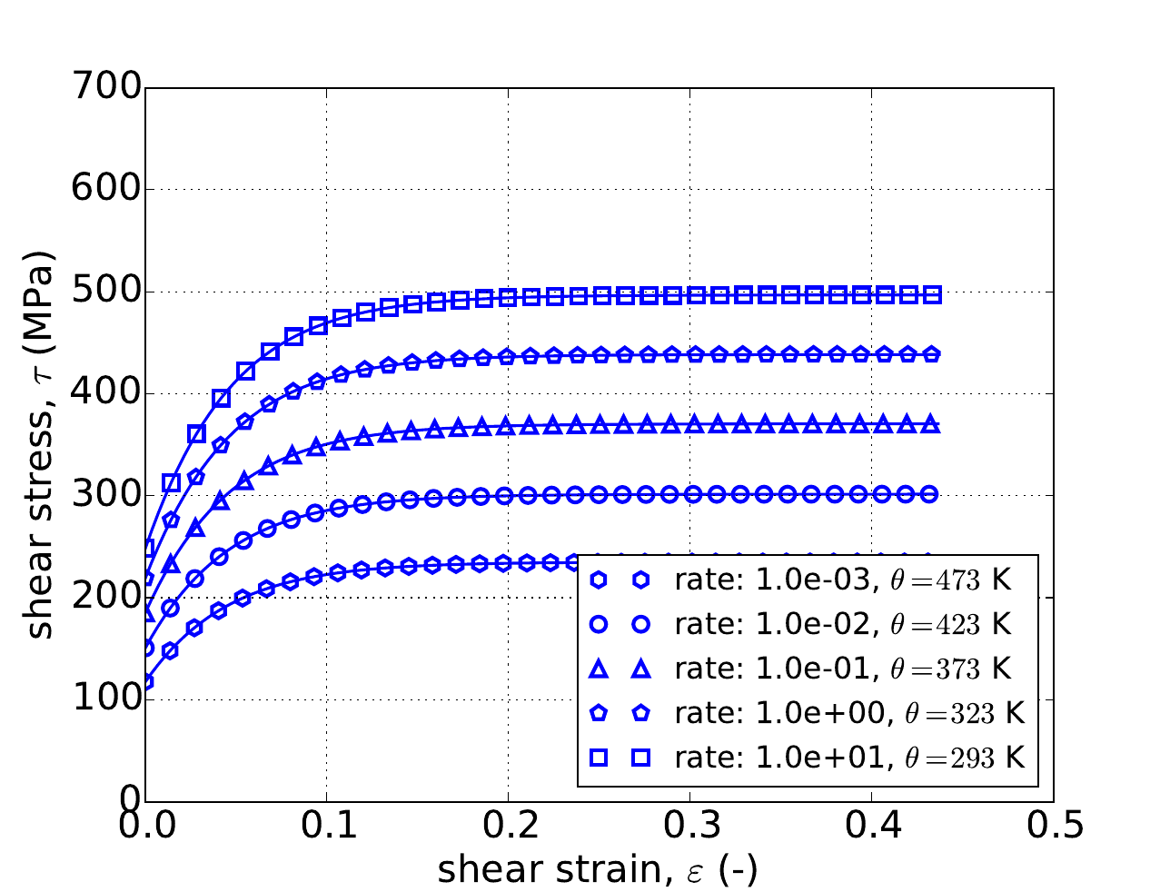
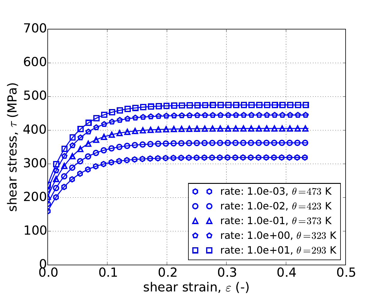
To complement the uniaxial results, pure shear results are given in Fig. 4.41. These results consider the same combinations of linear, power-law, and Voce isotropica hardening multiplier, Johnson-Cook and power-law breakdown rate multipliers, and Johnson-Cook temperature dependence. The same ranges of rates and temperatures are considered. As with the uniaxial cases, good agreement is noted between the analytical and numerical results.

Linear, Johnson-Cook

Linear, Power-Law Breakdown

Power-Law, Johnson-Cook

Power-Law, Power-Law Breakdown

Voce, Johnson-Cook

Voce, Power-Law Breakdown

Fig. 4.41 Pure shear responses of the \(J_2\) plasticity model using the flow-stress hardening model comprised of (a,b) linear, (c,d) power-law, and (e,f) Voce isotropic hardening, (a,c,e) Johnson-Cook and (b,d,f) Power-law breakdown rate multipliers and (a-f) Johnson-Cook temperature multipliers. Solid lines are analytical while open symbols are numerical (Sierra).

4.13.3.1.4. Decoupled Flow Stress

As a further extension, the verification of the decoupled flow-stress model is explored. To this end, Fig. 4.42 and Fig. 4.43 present uniaxial stress-strain results of various combinations of linear, power-law, and Voce isotropic hardening functions with rate-independent, Johnson-Cook, and power-law breakdown rate multipliers applied in different combinations to yield and hardening. Hardening is taken to be temperature-independent while yield has a Johnson-Cook temperature multiplier. The considered cases span five decades of applied strain rates and a range of temperatures. In these cases, the various analytical and numerical results are in agreement.

(L), Yield (JC) Hardening (PLB)

(L), Yield (-) Hardening (JC)

(L), Yield (PLB) Hardening (-)

(PL), Yield (JC) Hardening (PLB)

(PL), Yield (-) Hardening (JC)

(PL), Yield (PLB) Hardening (-)

Fig. 4.42 Uniaxial stress-strain responses of the \(J_2\) plasticity model using the decoupled flow-stress hardening model comprised of (a-c) linear (“L”) and (d-f) power-law (“PL”), (a-f) temperature independent hardening, (a-f) Johnson-Cook type temperature multiplier for yield, (a,d) Johnson-Cook (“JC”) and power-law breakdown (“PLB”) type yield and hardening rate multipliers, respectively, (b,e) rate-independent (-) yield with Johnson-Cook type hardening rate dependence, and (c,f) power-law breakdown yield rate dependence with rate-independent hardening. Solid lines are analytical while open symbols are numerical (Sierra).

(V), Yield (JC) Hardening (PLB)

(V), Yield (-) Hardening (JC)

(V), Yield (PLB) Hardening (i)

Fig. 4.43 Uniaxial stress-strain responses of the \(J_2\) plasticity model using the decoupled flow-stress hardening model comprised of (a-c) Voce isotropic hardening (“V”), (a-c) temperature independent hardening, (a-c) Johnson-Cook type temperature multiplier for yield, (a) Johnson-Cook (“JC”) and power-law breakdown (“PLB”) type yield and hardening rate multipliers, respectively, (b) rate-independent (-) yield with Johnson-Cook type hardening rate dependence, and (c) power-law breakdown yield rate dependence with rate-independent hardening. Solid lines are analytical while open symbols are numerical (Sierra).

While the previous results considered temperature-dependence on yield only, the temperature dependence on hardening is examined in Fig. 4.44 and Fig. 4.45. As with the previous case, linear, power-law, and Voce isotropic hardening laws are considered in conjunction with different combinations of Johnson-Cook, power-law breakdown, and rate-independent rate multipliers spanning large ranges of strain rates and temperatures. Once again, excellent agreement is noted between analytical and numerical results.

(L), Yield (JC) Hardening (PLB)

(L), Yield (-) Hardening (JC)

(L), Yield (PLB) Hardening (-)

(PL), Yield (JC) Hardening (PLB)

(PL), Yield (-) Hardening (JC)

(PL), Yield (PLB) Hardening (-)

Fig. 4.44 Uniaxial stress-strain responses of the \(J_2\) plasticity model using the decoupled flow-stress hardening model comprised of (a-c) linear (“L”) and (d-f) power-law (“PL”) hardening, (a-f) temperature independent yield, (a-f) Johnson-Cook type temperature multiplier for hardening, (a,d) power-law breakdown (“PLB”) and Johnson-Cook (“JC”) rate multipliers for yield and hardening, respectively (b,e) rate-independent (-)hardening with Johnson-Cook type yield rate dependence, and (c,f) power-law breakdown hardening rate dependence with rate-independent yield. Solid lines are analytical while open symbols are numerical (Sierra).

(V), Yield (JC) Hardening (PLB)

(V), Yield (-) Hardening (JC)

(V), Yield (PLB) Hardening (i)

Fig. 4.45 Uniaxial stress-strain responses of the \(J_2\) plasticity model using the decoupled flow-stress hardening model comprised of (a-c) Voce (“V”) isotropic hardening, (a-c) temperature independent yield, (a-c) Johnson-Cook type temperature multiplier for hardening, (a) power-law breakdown (“PLB”) and Johnson-Cook (“JC”) rate multipliers for yield and hardening, respectively (b) rate-independent (-)hardening with Johnson-Cook type yield rate dependence, and (c) power-law breakdown hardening rate dependence with rate-independent yield. Solid lines are analytical while open symbols are numerical (Sierra).

4.13.4. User Guide

BEGIN PARAMETERS FOR MODEL J2_PLASTICITY
  #
  # Elastic constants
  #
  YOUNGS MODULUS = <real>
  POISSONS RATIO = <real>
  SHEAR MODULUS  = <real>
  BULK MODULUS   = <real>
  LAMBDA         = <real>
  TWO MU         = <real>
  #
  # Yield surface parameters
  #
  YIELD STRESS = <real>
  BETA         = <real> (1.0)

#
  #
  # Hardening model
  #
  HARDENING MODEL = LINEAR | POWER_LAW | VOCE | USER_DEFINED |
  FLOW_STRESS | DECOUPLED_FLOW_STRESS | JOHNSON_COOK |
  POWER_LAW_BREAKDOWN
  #
  # Linear hardening
  #
  HARDENING MODULUS = <real>
  #
  # Power-law hardening
  #
  HARDENING CONSTANT = <real>
  HARDENING EXPONENT = <real> (0.5)
  LUDERS STRAIN      = <real> (0.0)
  #
  # Voce hardening
  #
  HARDENING MODULUS       = <real>
  EXPONENTIAL COEFFICIENT = <real>
  #
  # Johnson-Cook hardening
  #
  HARDENING FUNCTION = <string>hardening_function_name
  RATE CONSTANT      = <real>
  REFERENCE RATE     = <real>
  #
  # Power law breakdown hardening
  #
  HARDENING FUNCTION = <string>hardening_function_name
  RATE COEFFICIENT   = <real>
  RATE EXPONENT      = <real>
  # User defined hardening
  #
  HARDENING FUNCTION = <string>hardening_function_name
  #

#
  #
  # Following Commands Pertain to Flow_Stress Hardening Model
  #
  #    -  Isotropic Hardening model
  #
  ISOTROPIC HARDENING MODEL = LINEAR | POWER_LAW | VOCE |
                              USER_DEFINED
  #
  # Specifications for Linear, Power-law, and Voce same as above
  #
  # User defined hardening
  #
  ISOTROPIC HARDENING FUNCTION = <string>iso_hardening_fun_name
  #
  #     - Rate dependence
  #
  RATE MULTIPLIER = JOHNSON_COOK | POWER_LAW_BREAKDOWN |
     USER_DEFINED | RATE_INDEPENDENT (RATE_INDEPENDENT)
  #
  # Specifications for Johnson-Cook, Power-law-breakdown
  #     same as before EXCEPT no need to specify a
  #     hardening function
  #
  # User defined rate multiplier
  #
  RATE MULTIPLIER FUNCTION = <string> rate_mult_function_name
  #
  #     - Temperature dependence
  #
  TEMPERATURE MULTIPLIER = JOHNSON_COOK | USER_DEFINED |
     TEMPERATURE_INDEPENDENT (TEMPERATURE_INDEPENDENT)
  #
  #  Johnson-Cook temperature dependence
  #
  MELTING TEMPERATURE   = <real>
  REFERENCE TEMPERATURE = <real>
  TEMPERATURE EXPONENT  = <real>
  #
  #  User-defined temperature dependence
  TEMPERATURE MULTIPLIER FUNCTION = <string>temp_mult_function_name
  #
  # Following Commands Pertain to Decoupled_Flow_Stress Hardening Model
  #
  #    -  Isotropic Hardening model
  #
  ISOTROPIC HARDENING MODEL = LINEAR | POWER_LAW | VOCE | USER_DEFINED
  #
  # Specifications for Linear, Power-law, and Voce same as above
  #
  # User defined hardening
  #
  ISOTROPIC HARDENING FUNCTION = <string>isotropic_hardening_function_name
  #
  #     - Rate dependence
  #
  YIELD RATE MULTIPLIER = JOHNSON_COOK | POWER_LAW_BREAKDOWN |
              USER_DEFINED | RATE_INDEPENDENT (RATE_INDEPENDENT)
  #
  # Specifications for Johnson-Cook, Power-law-breakdown same as before
  #     EXCEPT no need to specify a hardening function
  #     AND should be preceded by YIELD
  #
  #     As an example for Johnson-Cook yield rate dependence,
  #
  YIELD RATE CONSTANT  = <real>
  YIELD REFERENCE RATE = <real>
  #
  # User defined rate multiplier
  #
  YIELD RATE MULTIPLIER FUNCTION = <string>yield_rate_mult_function_name
  #
  HARDENING_RATE MULTIPLIER = JOHNSON_COOK | POWER_LAW_BREAKDOWN |
              USER_DEFINED | RATE_INDEPENDENT (RATE_INDEPENDENT)
  #
  #     Syntax same as for yield parameters but with a HARDENING prefix
  #
  #     - Temperature dependence
  #
  YIELD TEMPERATURE MULTIPLIER = JOHNSON_COOK | USER_DEFINED |
            TEMPERATURE_INDEPENDENT (TEMPERATURE_INDEPENDENT)
  #
  #  Johnson-Cook temperature dependence
  #
  YIELD MELTING TEMPERATURE   = <real>
  YIELD REFERENCE TEMPERATURE = <real>
  YIELD TEMPERATURE EXPONENT  = <real>
  #
  #  User-defined temperature dependence
  YIELD TEMPERATURE MULTIPLIER FUNCTION = <string>yield_temp_mult_fun_name
  #
  HARDENING TEMPERATURE MULTIPLIER = JOHNSON_COOK | USER_DEFINED |
            TEMPERATURE_INDEPENDENT (TEMPERATURE_INDEPENDENT)
  #
  #   Syntax for hardening constants same as for yield but
  #            with HARDENING prefix

#
  #
  # Optional Failure Definitions
  #    Following only need to be defined if intend to use failure model
  #
  FAILURE MODEL = TEARING_PARAMETER | JOHNSON_COOK_FAILURE | WILKINS
                  | MODULAR_FAILURE | MODULAR_BCJ_FAILURE

  CRITICAL FAILURE PARAMETER = <real>
  #
  # TEARING_PARAMETER Failure model definitions
  #
  TEARING PARAMETER EXPONENT = <real>
  #
  # JOHNSON_COOK_FAILURE Failure model definitions
  #
  JOHNSON COOK D1       = <real>
  JOHNSON COOK D2       = <real>
  JOHNSON COOK D3       = <real>
  JOHNSON COOK D4       = <real>
  JOHNSON COOK D5       = <real>
  #
  #Following Johnson-Cook parameters can only be defined once.  As such, only
  #  needed if not previously defined via Johnson-Cook multipliers
  #  w/ flow-stress hardening.  Does need to be defined
  #  w/ Decoupled Flow Stress
  #
  REFERENCE RATE        = <real>
  REFERENCE TEMPERATURE = <real>
  MELTING TEMPERATURE   = <real>
  #
  # WILKINS Failure model definitions
  #
  WILKINS ALPHA    = <real>
  WILKINS BETA     = <real>
  WILKINS PRESSURE = <real>
  #
  #  MODULAR_FAILURE Failure model definitions
  #
  PRESSURE MULTIPLIER         = PRESSURE_INDEPENDENT | WILKINS
                                | USER_DEFINED (PRESSURE_INDEPENDENT)
  LODE ANGLE MULTIPLIER       = LODE_ANGLE_INDEPENDENT |
                                WILKINS (LODE_ANGLE_INDEPENDENT)
  TRIAXIALITY MULTIPLIER      = TRIAXIALITY_INDEPENDENT | JOHNSON_COOK
                                | USER_DEFINED (TRIAXIALITY_INDEPENDENT)
  RATE FAIL MULTIPLIER        = RATE_INDEPENDENT | JOHNSON_COOK
                                | USER_DEFINED (RATE_INDEPENDENT)
  TEMPERATURE FAIL MULTIPLIER = TEMPERATURE_INDEPENDENT | JOHNSON_COOK
                                | USER_DEFINED (TEMPERATURE_INDEPENDENT)
  #
  # Individual multiplier definitions
  #
  PRESSURE MULTIPLIER = WILKINS
  WILKINS ALPHA       = <real>
  WILKINS PRESSURE    = <real>
  #
  PRESSURE MULTIPLIER = USER_DEFINED
  PRESSURE MULTIPLIER FUNCTION = <string> pressure_multiplier_fun_name
  #
  LODE ANGLE MULTIPLIER = WILKINS
  WILKINS BETA          = <real>
  #
  TRIAXIALITY MULTIPLIER = JOHNSON_COOK
  JOHNSON COOK D1        = <real>
  JOHNSON COOK D2        = <real>
  JOHNSON COOK D3        = <real>
  #
  TRIAXIALITY MULTIPLIER = USER_DEFINED
  TRIAXIALITY MULTIPLIER FUNCTION = <string> triaxiality_multiplier_fun_name
  #
  RATE FAIL MULTIPLIER = JOHNSON_COOK
  JOHNSON COOK D4      = <real>
  # REFERENCE RATE should only be added if not previously defined
  REFERENCE RATE       = <real>
  #
  RATE FAIL MULTIPLIER = USER_DEFINED
  RATE FAIL MULTIPLIER FUNCTION = <string> rate_fail_multiplier_fun_name
  #
  TEMPERATURE FAIL MULTIPLIER = JOHNSON_COOK
  JOHNSON COOK D5             = <real>
  # JC Temperatures should only be defined if not previously given
  REFERENCE TEMPERATURE       = <real>
  MELTING TEMPERATURE         = <real>
  #
  TEMPERATURE FAIL MULTIPLIER          = USER_DEFINED
  TEMPERATURE FAIL MULTIPLIER FUNCTION = <string> temp_multiplier_fun_name
  #
  # MODULAR_BCJ_FAILURE Failure model definitions
  #
  INITIAL DAMAGE    = <real>
  INITIAL VOID SIZE = <real>
  DAMAGE BETA       = <real> (0.5)
  GROWTH MODEL      = COCKS_ASHBY | NO_GROWTH (NO_GROWTH)
  NUCLEATION MODEL  = HORSTEMEYER_GOKHALE | CHU_NEEDLEMAN_STRAIN
                      | NO_NUCLEATION (NO_NUCLEATION)
  #
  GROWTH RATE FAIL MULTIPLIER        = JOHNSON_COOK | USER_DEFINED
                                       | RATE_INDEPENDENT
                                       (RATE_INDEPENDENT)
  GROWTH TEMPERATURE FAIL MULTIPLIER = JOHNSON_COOK | USER_DEFINED
                                       | TEMPERATURE_INDEPENDENT
                                       (TEMPERATURE_INDEPENDENT)
  #
  NUCLEATION RATE FAIL MULTIPLIER        = JOHNSON_COOK | USER_DEFINED
                                           | RATE_INDEPENDENT
                                           (RATE_INDEPENDENT)
  NUCLEATION TEMPERATURE FAIL MULTIPLIER = JOHNSON_COOK | USER_DEFINED
                                           | TEMPERATURE_INDEPENDENT
                                           (TEMPERATURE_INDEPENDENT)
  #
  # Definitions for individual growth and nucleation models
  #
  GROWTH MODEL = COCKS_ASHBY
  DAMAGE EXPONENT = <real> (0.5)
  #
  NUCLEATION MODEL      = HORSTEMEYER_GOKHALE
  NUCLEATION PARAMETER1 = <real> (0.0)
  NUCLEATION PARAMETER2 = <real> (0.0)
  NUCLEATION PARAMETER3 = <real> (0.0)
  #
  NUCLEATION MODEL          = CHU_NEEDLEMAN_STRAIN
  NUCLEATION AMPLITUDE      = <real>
  MEAN NUCLEATION STRAIN    = <real>
  NUCLEATION STRAIN STD DEV = <real>
  #
  # Definitions for rate and temperature fail multiplier
  #   Note: only showing definitions for growth.
  #    Nucleation terms are the same just with NUCLEATION instead
  #    of GROWTH
  #
  GROWTH RATE FAIL MULTIPLIER = JOHNSON_COOK
  GROWTH JOHNSON COOK D4      = <real>
  GROWTH REFERENCE RATE       = <real>
  #
  GROWTH RATE FAIL MULTIPLIER          = USER_DEFINED
  GROWTH RATE FAIL MULTIPLIER FUNCTION = <string> growth_rate_fail_mult_func
  #
  GROWTH TEMPERATURE FAIL MULTIPLIER = JOHNSON_COOK
  GROWTH JOHNSON COOK D5             = <real>
  GROWTH REFERENCE TEMPERATURE       = <real>
  GROWTH MELTING TEMPERATURE         = <real>
  #
  GROWTH TEMPERATURE FAIL MULTIPLIER          = USER_DEFINED
  GROWTH TEMPERATURE FAIL MULTIPLIER FUNCTION = <string> temp_fail_mult_func
  #

#
  #
  # Optional Adiabatic Heating/Thermal Softening  Definitions
  #    Following only need to be defined if intend to use failure model
  #
  THERMAL SOFTENING MODEL = ADIABATIC | COUPLED
  #
  SPECIFIC HEAT = <real> # not needed for COUPLED
  BETA_TQ       = <real>

END [PARAMETERS FOR MODEL J2_PLASTICITY]

In the command blocks that define the \(J_2\) plasticity model:

• The reference nominal yield stress, \(\bar{\sigma}\), is defined with the YIELD STRESS command line.

• The beta parameter defines if hardening is isotropic.

• The type of hardening law is defined with the HARDENING MODEL command line, other hardening commands then define the specific shape of that hardening curve.

• The hardening modulus for a linear hardening model is defined with the HARDENING MODULUS command line.

• The hardening constant for a power law hardening model is defined with the HARDENING CONSTANT command line.

• The hardening exponent for a power law hardening model is defined with the HARDENING EXPONENT command line.

• The Luders strain for a power law hardening model is defined with the LUDERS STRAIN command line.

• The hardening function for a user defined hardening model is defined with the HARDENING FUNCTION command line.

• The shape of the spline for the spline based hardening is defined by the CUBIC SPLINE TYPE, CARDINAL PARAMETER, KNOT EQPS, and KNOT STRESS command lines.

• The isotropic hardening model for the flow stress hardening model is defined with the ISOTROPIC HARDENING MODEL command line.

• The function name of a user-defined isotropic hardening model is defined via the ISOTROPIC HARDENING FUNCTION command line.

• The optional rate multiplier for the flow stress hardening model is defined with the RATE MULTIPLIER command line.

• The optional temperature multiplier for the flow stress hardening model is defined via the TEMPERATURE MULTIPLIER command line.

• The function name of a user-defined temperature multiplier is defined with the TEMPERATURE MULTIPLIER FUNCTION command line.

• For a Johnson-Cook temperature multiplier, the melting temperature, \(\theta_{\text{melt}}\), is defined via the MELTING TEMPERATURE command line.

• For a Johnson-Cook temperature multiplier, the reference temperature, \(\theta_{\text{ref}}\), is defined via the REFERENCE TEMPERATURE command line.

• For a Johnson-Cook temperature multiplier, the temperature exponent, \(M\), is defined via the TEMPERATURE EXPONENT command line.

• The optional rate multiplier for the yield stress for the decoupled flow stress hardening model is defined with the YIELD RATE MULTIPLIER command line.

• The optional rate multiplier for the hardening for the decoupled flow stress hardening model is defined with the HARDENING RATE MULTIPLIER command line.

• The optional temperature multiplier for the yield stress for the decoupled flow stress hardening model is defined with the YIELD TEMPERATURE MULTIPLIER command line.

• The optional temperature multiplier for the hardening for the decoupled flow stress hardening model is defined via the HARDENING TEMPERATURE MULTIPLIER command line.

Output variables available for this model are listed in Table 4.17.

Table 4.17 State Variables for J2 PLASTICITY Model

Name	Description
EQPS	equivalent plastic strain, \(\bar{\varepsilon}^{p}\)
EQDOT	equivalent plastic strain rate, \(\dot{\bar{\varepsilon}}^{p}\)
SEFF	effective stress, \(\phi\)
TENSILE_EQPS	tensile equivalent plastic strain, \(\bar{\varepsilon}^{p}_{t}\)
DAMAGE	damage, \(\phi\)
VOID_COUNT	void count, \(\eta\)
VOID_SIZE	void size, \(\upsilon\)
DAMAGE_DOT	damage rate, \(\dot{\phi}\)
VOID_COUNT_DOT	void count rate, \(\dot{\eta}\)
PLASTIC_WORK_HEAT_RATE	plastic work heat rate, \(\dot{Q}^p\)

---

[1] (1,2,3,4,5,6)

G.R. Johnson and W.H. Cook. A constitutive model and data for metals subjected to large strains, high strain rates and high temperatures. In Proc. 7th. Int. Symp. on Ballistics, 541–547. The Hague, The Netherlands, 1983.

[2] (1,2,3,4,5,6)

G.R. Johnson and W.H. Cook. Fracture characteristics of three metals subjected to various strains, strain rates, temperatures and pressures. Engineering Fracture Mechanics, 21(1):31–48, 1985.

[3] (1,2)

B.T. Lester and W.M. Scherzinger. Failure formulations in modular plasticity models. Memo to distribution SAND2019-9678R, Sandia National Laboratories, Albuquerque, NM and Livermore, CA, 2019.

[4] (1,2)

B.T. Lester and W.M. Scherzinger. Modular growth and nucleation formulations in modular plasticity models. Memo to distribution SAND2020-7404R, Sandia National Laboratories, Albuquerque, NM and Livermore, CA, 2020.

[5] (1,2)

B.T. Lester and W.M. Scherzinger. Adiabatic heating in modular plasticity models. Memo to distribution SAND2019-15003R, Sandia National Laboratories, Albuquerque, NM and Livermore, CA, 2019.

[6]

R. Hill. The Mathematical Theory of Plasticity. Oxford University Press, 1950.

[7]

J. Lemaitre and J.-L. Chaboche. Mechanics of Solid Materials. Cambridge University Press, 1990.

[8]

J. Lubliner. Plasticity Theory. Dover, 2008.

[9]

H. J. Frost and M. F. Ashby. Deformation Mechanism Maps: the Plasticity and Creep of Metals and Ceramics. Pergamon Press, 1982.

[10]

A.A. Brown and D.J. Bammann. Validation of a model for static and dynamic recrystallization in metals. International Journal of Plasticity, 32–33:17–35, 2012.