4.29. Foam Damage Model

4.29.1. Theory

The foam damage model was developed at Sandia National Laboratories to model the behavior of rigid polyurethane foams under a variety of loading conditions [[1]]. For instance, temperature, rate, and tension-compression dependencies are all built into this model. This model, leverages previous efforts and experience with other foam models (e.g. low density foam Section 4.26, foam plasticity Section 4.27, and viscoplastic foam Section 4.28). Like those past efforts, this model utilizes an additive decomposition of the strain rates into elastic and inelastic parts,

\[D_{ij} = D_{ij}^{\text{e}} + D_{ij}^{\text{in}}.\]

It is also assumed that the elastic response is linear and isotropic such that the stress rate for isothermal conditions is given by the following equation

\[\stackrel{\circ}{\sigma}_{ij} = \mathbb{C}_{ijkl}D_{kl}^{\text{e}} = \mathbb{C}_{ijkl}\left( D_{kl} - D_{kl}^{\text{in}} \right),\]

with \(\mathbb{C}_{ijkl}\) being the fourth-order, isotropic elasticity tensor. The specific stress rate considered is arbitrary as long as it is object. Two common rates satisfying that constraint are the Jaumann and Green-McInnis rates.

The initial yield surface is assumed to be an ellipsoid about the hydrostat and is described by the function

(4.139)\[f = \frac{\bar{\sigma}^{2}}{a^{2}} + \frac{p^{2}}{b^{2}} - 1 = 0,\]

where \(a\) and \(b\) are state variables that define the current deviatoric and volumetric strengths, respectively, of the foam. The von Mises effective stress, \(\bar{\sigma}\) is a scalar measure of the deviatoric stress given by

\[\bar{\sigma} = \sqrt{\frac{3}{2} s_{ij}s_{ij}},\]

while \(p\) is the pressure, or mean stress, and is defined as

\[p = \frac{1}{3} \sigma_{kk},\]

with \(\sigma_{ij}\) and \(s_{ij}\) being the components of the Cauchy and deviatoric stress. This latter tensor may be written as,

\[s_{ij} = \sigma_{ij} - p \delta_{ij},\]

where \(\delta_{ij}\) are the components of the identity tensor - \(\delta_{ij} = 1\) if \(i=j\), \(\delta_{ij} = 0\) if \(i \neq j\).

For this model, the yield function (4.139) is re-written as

\[f = \sigma^{*} - a = 0\]

with the effective stress, \(\sigma^{*}\), being a function of the von Mises effective stress, \(\bar\sigma\), and the pressure, \(p\), as follows

\[\sigma^{*} = \sqrt{\bar{\sigma}^{2} + \frac{a^{2}}{b^{2}} p^{2}}.\]

Next, using a Perzyna-type formulation, the following expression for the inelastic strain rate, \(D_{ij}^{\text{in}}\), is developed

\[\begin{split}D_{ij}^{\text{in}} = \begin{cases} \displaystyle \dot{\bar{\varepsilon}}^p \, g_{ij} = e^{h}\left( \frac{\sigma^{*}}{a}-1\right)^{n} g_{ij} & \displaystyle \text{ if } \; \frac{\sigma^{*}}{a} - 1 > 0 \\ \displaystyle 0 & \displaystyle \text{ if } \; \frac{\sigma^{*}}{a} - 1 \leq 0, \end{cases}\end{split}\]

where \(g_{ij}\) are the components of a symmetric, second-order tensor that defines the orientation of the inelastic flow. This type of model is sometimes referred to as an over-stress model because the inelastic rate is a function of the over-stress - the distance outside the yield surface. For associated flow, \(g_{ij}\) is simply normal to the yield surface and is given by

(4.140)\[g_{ij}^{\text{a}} = \frac{\displaystyle\frac{\partial f}{\partial \sigma_{ij}}}{\displaystyle \left|\frac{\partial f}{\partial{\sigma_{kl}}}\right|} = \frac{\displaystyle \frac{3}{a^{2}} s_{ij} + \frac{2}{3b^{2}} p \, \delta_{ij}}{\displaystyle \left| \frac{3}{a^{2}} s_{kl} + \frac{2}{3b^{2}} p \, \delta_{kl} \right|}.\]

When lower density foams are subjected to a simple load path like uniaxial compression, the inelastic flow direction at moderate strains appears nearly uniaxial. In other words, the flow direction is given by the normalized stress tensor as follows

\[g_{ij}^{\text{r}} = \frac{\sigma_{ij}}{\left| {\sigma_{kl}} \right|}.\]

This type of flow is called radial flow. The foam damage model has another parameter, \(\beta\), which allows for the flow direction to be prescribed as a linear combination of associated and radial flow such that,

(4.141)\[g_{ij} = \frac{(1-\beta) \, g_{ij}^{\text{a}} + \beta \, g_{ij}^{\text{r}}}{\left| (1-\beta) \, g_{kl}^{\text{a}} + \beta \, g^{\text{r}}_{kl} \right|}.\]

Rigid polyurethane foams have little ductility when they are subjected to tensile stress. For this loading case, the materials behave more like brittle materials and even for uniaxial compression the foams often show cracking at large strains.

The damage surfaces for the foam damage model are simply three orthogonal planes with the normals given by the positive principal stress axes. The damage surfaces are given by the following equation

\[f^{i}_{\text{dam}} = \hat\sigma^{i} - c \left( 1 - w \right), \;\;\; ; \;\;\; i = 1,2,3\]

where \(\hat{\sigma}^{i}\) is a principal stress, \(c\) is the initial tensile strength which is a material parameter, and \(w\) is a scalar measure of the damage. As damage occurs, the damage surface will collapse toward the origin and the foam will lose tensile strength. The foam will, however, still have compressive strength.

Damage is taken to be a positive, monotonically increasing function of the damage strain, \(\varepsilon_{\text{dam}}\), and the damage strain is a function of the maximum principal strain, \(\varepsilon_{\text{max}}\), and the plastic volume strain, \(\varepsilon^{\text{p}}_{v}\), such that

\[w = w\left( \varepsilon_{\text{dam}} \right) \;\;\; ; \;\;\; \varepsilon_{\text{dam}} = a_{\text{dam}}\varepsilon_{\text{max}} + b_{\text{dam}}\varepsilon_{v}^{\text{p}},\]

with the material parameters \(a_{\text{dam}}\) and \(b_{\text{dam}}\) controlling the rate at which damage is generated in tension and compression, respectively. The model does not allow healing, so the damage never decreases even if the damage strain decreases.

To fully capture temperature, strain rate, and lock-up effects, several material parameters are defined as functions of temperature, \(\theta\), and/or some measure of the amount of compaction, e.g. the maximum volume fraction of the solid material obtained during any prior loading, \(\phi\). For instance,

\[\begin{split}E \left( \theta, \phi \right) & = E \, h_{E}\left( \theta \right) \, f_{E} \left( \phi \right), \nonumber \\ \\ \nu \left( \theta, \phi \right) & = \nu \, h_{\nu}\left( \theta \right) \, f_{\nu} \left( \phi \right), \nonumber\end{split}\]

and the natural logarithm of the reference flow rate, \(h\), and the power law exponent, \(n\) are also functions of temperature

\[\begin{split}h \left( \theta \right) & = h \, h_{h}\left( \theta \right) \nonumber \\ \\ n \left( \theta \right) & = n \, h_{n}\left( \theta \right). \nonumber\end{split}\]

The current deviatoric and volumetric strengths are hardening functions of the maximum volume fraction of the solid material obtained during any prior loading, \(\phi\), as is the parameter that defines the fraction of associated and radial flow, \(\beta\). Therefore,

\[\begin{split}a = a \left( \phi \right) \;\;\; ; \;\;\; b = b \left( \phi \right) \nonumber \\ \\ \beta = \beta \left( \phi \right). \nonumber\end{split}\]

Through the loading cycle, the maximum volume fraction of solid material is written as,

\[\phi=\max_{t>0}\tilde{\phi}\left(t\right)\]

where \(\tilde{\phi}\left(t\right)\) is the current volume faction of solid material defined as

\[\tilde{\phi}\left(t\right)=\frac{\phi_0}{\exp\left(\varepsilon^{\text{p}}_v\right)},\]

with \(\phi_0\) and \(\varepsilon^{\text{p}}_v\) being the initial solid volume fraction and plastic volumetric strain, respectively.

The foam damage model, as presented, provides a phenomenological model with enough flexibility to model the observed deformation and failure of rigid polyurethane foams.

4.29.2. Implementation

Like the other foam models, the foam damage model is integrated using an explicit forward Euler scheme. Essentially, this specific form is a combination of a rate-dependent viscoplastic mechanism and a distinct damage element. At the highest level, these two responses are considered independently and sequentially with the viscoplastic behavior being evaluated first. Initially, the damage parameter is set to 0 and is limited to a maximum value of 0.99 to prevent the tensile strength from going to zero or negative due to numerical round-off. Foam material elements that are completely damaged can be removed using element death based approaches in the case of the damage variable reaching a value close to 1, say 0.99. This topic, however, will not be discussed here as the focus is on the constitutive behavior of the foam model.

To ensure integration stability, an allowable strain increment is first calculated so that a critical time step may be found. Essentially, such a maximum is given by the ratio of shear strength to elastic modulus. If the input time step is sufficiently small to meet this requirement, the material state at time \(t=t_{n+1}\) is calculated directly. For unsuitably large time steps, a series of sub-increments are used such that the integration may proceed in a stable fashion. Specifically, a total time step of \(\Delta t\) is subdivided into \(N\) sub-increments with the \(k^{th}\) such sub-increment having a time interval of \(\delta t^k\) so that \(\Delta t=\sum_{k=1}^N\delta t^k\). In this case, the same forward Euler scheme is used to integrate successively over the sub-increments. For temperature dependent properties (e.g. the power law exponent \(n\)), the value at the start of the sub-increment is determined by linearly interpolating over the total time step,

\[n^k=n_n+\frac{\Delta t^k}{\Delta t}\left(n_{n+1}-n_{n}\right),\]

with \(\Delta t^k\) begin the current sub-increment time step, \(\Delta t^k=\sum_{r=1}^k \delta t^r\). For simplicity, in the remainder of this section it is assumed that the input time step is acceptable and only a single increment is needed. If additional sub-increments are needed, the below steps would be repeated \(N\) times with time intervals of \(\delta t^k\).

The rate-dependent plastic response is then calculated in a fashion very similar to that of the viscoplastic foam model (Section 4.28.2). The key differences are primarily the additional, and more complex, dependencies of \(\nu,~\beta,~a,\) and \(b\) on the solid volume fraction. As such, first the various material properties and model parameters that are dependent on temperature, \(\theta\), or solid volume fraction, \(\phi\), are determined based on the respective values at \(t=t_n\). The effective plastic strain rate, \(\dot{\bar{\varepsilon}}^p\), is readily found as,

\[\dot{\bar{\varepsilon}}^p=e^{h\left(\theta_n\right)}\left<\frac{\sigma_n^*}{a\left(\phi_n\right)}-1\right>^{n\left(\theta_n\right)},\]

where \(\sigma_n^*\) is given by,

\[\sigma_n^*=\sqrt{\bar{\sigma}^2_n+\frac{a^2\left(\phi_n\right)}{b^2\left(\phi_n\right)}p_n^2},\]

and \(\left< x\right>\) are the Macaulay brackets evaluated as,

\[\begin{split}\left<x\right>=\left\{\begin{array}{cc} x, & x \geq 0 \\ 0, & x < 0 \end{array} \right. .\end{split}\]

Knowing the effective plastic strain increment, corresponding stress increments may be determined. Specifically, the rates of change of the deviatoric stress, \(\dot{s}_{ij}\), and pressure, \(\dot{p}\), are given for isothermal conditions by

\[\begin{split}\dot{s}_{ij}=2\mu_n\left(\hat{d}_{ij}-\hat{d}^{\text{p}}_{ij}\right), \\ \dot{p}=K_n\left(d_{kk}-d^{\text{p}}_{kk}\right),\end{split}\]

with \(d_{ij}\) and \(d^{\text{p}}_{ij}\) being the the total and plastic, respectively, rates of deformation, and the symbol \(\hat{x}_{ij}\) denoting the deviatoric part of the tensor \(x_{ij}\). The plastic strain rate is given by,

\[d^{\text{p}}_{ij}=\dot{\bar{\varepsilon}}^pg_{ij}^n,\]

where \(g_{ij}^n\) is evaluated via relation (4.140)-(4.141) using state variable at time \(t=t_n\) and it is noted that \(\beta=\beta\left(\phi_n\right)\). Elastic constants \(K_n\) and \(\mu_n\) are found through isotropic relations using the values \(E_n\) and \(\nu_n\) so the temperature and solid volume fraction dependencies may be incorporated.

Therefore, after accounting for plastic deformation and any associated temperature changes,

\[\begin{split}\tilde{s}_{ij} & = \frac{\mu_{n+1}}{\mu_n}s_{ij}^n+\dot{s}_{ij} \Delta t, \\ \tilde{p}_{ij} & = \frac{K_{n+1}}{K_{n}}p^n+\dot{p}\Delta t, \\ \tilde{T}_{ij} & = \tilde{s}_{ij}+\tilde{p}\delta_{ij},\end{split}\]

where the tilde, \(\tilde{x}\), is used to distinguish the fact that the damage response has not yet been evaluated and these are temporary variables. Updated expressions for the state variables are also given as,

\[\begin{split}\varepsilon^{\text{p}-n+1}_v & = \varepsilon^{\text{p}-n}_v+d^{\text{p}}_{kk}\Delta t, \\ \phi_{n+1} & = \max\left[\frac{\phi_0}{\exp\left(\varepsilon^{\text{p}-n+1}_v\right)},\phi_n \right].\end{split}\]

With the plastic deformations determined, the damage state of the material is evaluated. As a first step, the eigenvalues, \(\hat{\sigma}^i\), and vectors, \(\hat{e}^k_i\) (where \(k\) denotes the corresponding eigenvalue) of the stress state, \(\tilde{T}_{ij}\), and eigenvalues, \(\varepsilon_i\) of the total strain state are determined. Of particular interest is the maximum eigenvalue of the strain tensor, \(\varepsilon_{\text{max}}\). The damage strain, \(\varepsilon_{\text{dam}}^{n+1}\), is

\[\varepsilon_{\text{dam}}^{n+1}=\left< a_{\text{dam}}\varepsilon_{\text{max}}+b_{\text{dam}}\varepsilon^{\text{p}-n+1}_v \right>,\]

with \(\left<\right>\) being Macaulay brackets. This value of the damage strain is then used to evaluate the current value of the damage, \(w^{n+1}\), and a check is also imposed to insure that the damage does not decrease. An effective tensile strength, \(\sigma^{\text{dam}}\), may then be calculated as

\[\sigma^{\text{dam}}=c\left(1-w^{n+1}\right),\]

leading to a damage surface of the form,

\[f^i_{\text{dam}}=\hat{\sigma}^i-\sigma^{\text{dam}}.\]

The eigenvalues of the updated stress tensor may be written as,

\[\begin{split}\hat{\sigma}^i_{n+1}=\left\{\begin{array}{cc} \hat{\sigma}^i, & f^i_{\text{dam}} \leq 0 \\ \sigma^{\text{dam}}, & f^i_{\text{dam}} > 0 \end{array}\right. ,\end{split}\]

producing a final updated stress state of the form,

\[T^{n+1}_{ij}=\sum_{k=1}^3\hat{\sigma}^k_{n+1}\hat{e}^k_i\hat{e}^k_j.\]

4.29.3. Verification

Given the complexity and variety of response and features of the foam damage model, a series of verification analyses are performed. Common material properties and model parameters used for these investigations are given in Table 4.45. For these initial studies, isothermal loadings are considered and the solid volume fraction dependence of the elastic properties is neglected (\(f_{E}\left(\phi\right)=1,\ f_{\nu}\left(\phi\right)=1\)). Properties used correspond to those of a FR3712 foam from [[1]]. In the case of the elastic modulus, flow rate, and exponent, the values correspond those at a temperature of 18.30\({}^\circ\)C.

Table 4.45 Common material properties and model parameters for the foam damage model used during verification testing.

\(E\)	9,240 psi	\(c\)	280 psi
\(\nu\)	0.25	\(a_{\text{dam}}\)	1.0
\(h\)	2.60	\(b_{\text{dam}}\)	0.55
\(n\)	14.0	\(\phi_0\)	0.160

The shear strength, hydrostatic strength, and damage function all require user defined functional forms. For purposes of these tests, simple linear forms are considered for use in the analytical evaluations. Using the data same FR3712 data as before, simplified expressions of the form,

\[\begin{split}a\left(\phi\right) & = 160 + 2400\phi, \\ b\left(\phi\right) & = 160+3266.67\phi, \\ w\left(\varepsilon_{\text{dam}}\right) & = \frac{10}{3}\varepsilon_{\text{dam}},\end{split}\]

are considered.

4.29.3.1. Uniaxial Compression

First, the behavior of the model subject to a uniaxial compression load is considered. As the loading is purely compressive, no tensile stress is generated and the damage surface is not violated. Therefore, only the rate-dependent plasticity is considered in this section. Given the rate-dependent nature, no analytical solution is readily available and and a semi-analytical approach is developed by specializing the equations to uniaxial compression. Additionally, it is noted that the flow parameter, \(\beta\), is not specified above and is enabled in this model to be an user-defined function of the solid volume fraction \(\phi\). Here, to isolate the impact of this parameter, the two extreme cases are considered – fully associated or radial flow with \(\beta=0,~1\), respectively.

To induce the uniaxial stress state of interest, a displacement of the form \(u_1=\lambda_1\) is applied while the remaining degrees of freedom (2 and 3) are left traction free. The applied displacement scales linearly from \(\lambda_1=0\) at \(t=0.0\) to \(\lambda_1=-0.7\) at \(t=1.0\). In this case, the stress state is simply \(\sigma_{ij}=\sigma_{11}\delta_{i1}\delta_{j1}\) leading to an overstress of the form \(\sigma^*=|\sigma_{11}|\sqrt{1+\frac{a^2}{9b^2}}\). For both associated and radial flow, the inelastic flow rate simplifies to,

\[D_{ij}^{\text{in}}=e^h\left<\frac{|\sigma_{11}|}{3ab}\sqrt{a^2+9b^2}-1\right>^ng_{ij},\]

with \(\left< \cdot\right>\) being Macaulay brackets. The total strains may then be written as,

\[\begin{split}\varepsilon_{11} & = \ln\left(1+\lambda_1\right), \\ \varepsilon_{22}=\varepsilon_{33} & = -\nu\left(\ln\left(1+\lambda_1\right)-\varepsilon_{11}^{\text{in}}\right)+\varepsilon_{22}^{\text{in}},\end{split}\]

where \(\varepsilon^{\text{in}}_{ij}=\int_{0}^t D_{ij}^{\text{in}}d\tau\). The associated and radial flow cases are distinguished by the form of \(g_{ij}\). In the latter case, \(g_{ij}\) reduces simply to \(g_{ij}^{\text{r}}=\delta_{i1}\delta_{j1}\). The former case, on the other hand, produces a flow direction of the form,

\[\begin{split}\hat{g} & = \frac{1}{3\sqrt{\frac{2}{3}\left(2a^4+81b^4\right)}}, \\ g^{\text{r}}_{11} & = \hat{g}2\left(a^2+9b^2\right), \\ g^{\text{r}}_{22} = g^{\text{r}}_{33} & = \hat{g}\left(2a^2-9b^2\right) .\end{split}\]

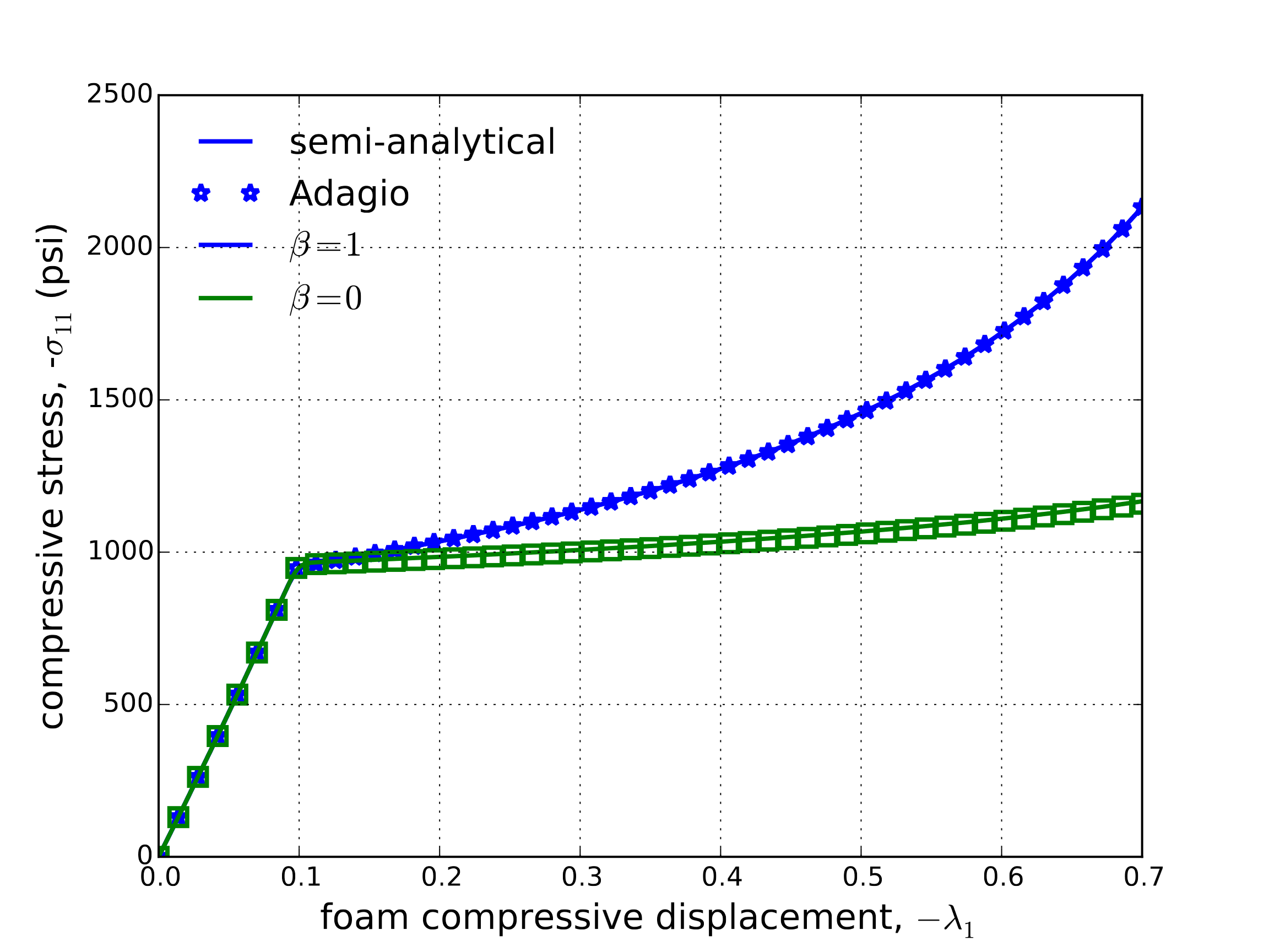
The stress evolution for both of these flow cases determined numerically (adagio) and semi-analytically is presented in Fig. 4.126.

Axial stress

Solid volume fraction

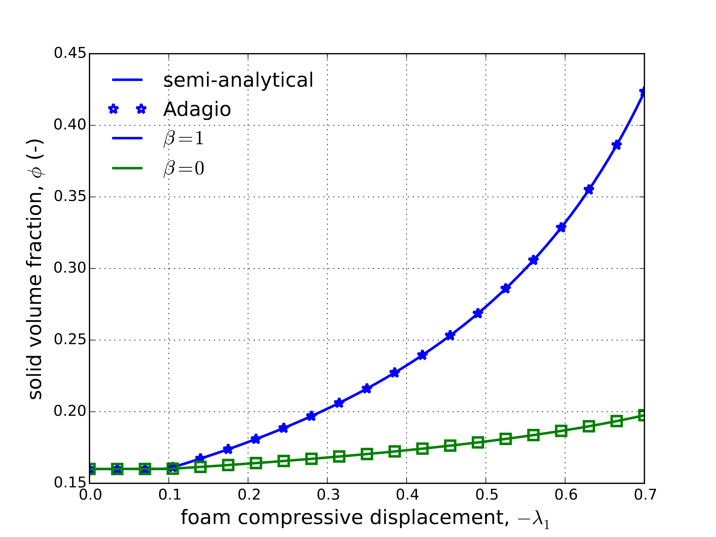
Fig. 4.126 Axial stress (a) and maximum solid volume fraction (b), \(\phi\), evolution obtained as a function of applied compressive displacement and determined via the foam damage model considering both associated (\(\beta=0\)) and radial(\(\beta=1\)) flow assumptions semi-analytically and numerically.

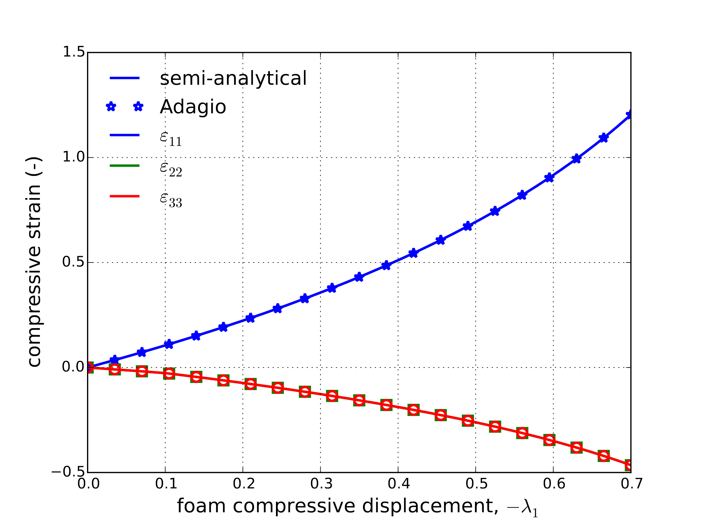
From these results, the impact of the flow direction choice can be observed to have a large impact on the model response. Specifically, in the radial case more substantial hardening is seen throughout the entire plastic domain. As the hardening results from the solid volume fraction (which is a function of volumetric plastic deformation), such a difference may be anticipated. Specifically, given the uniaxial plastic flow in the radial case more pronounced volumetric strains are to be expected. The associated case, on the other hand, has a more deviatoric character leading to lower plastic volume strains. This difference may also be more readily observed in the total strain evolutions of the associated and radial cases in Fig. 4.127(a) and Fig. 4.127(b), respectively.

Associated Flow, beta=0

Radial Flow, beta=1

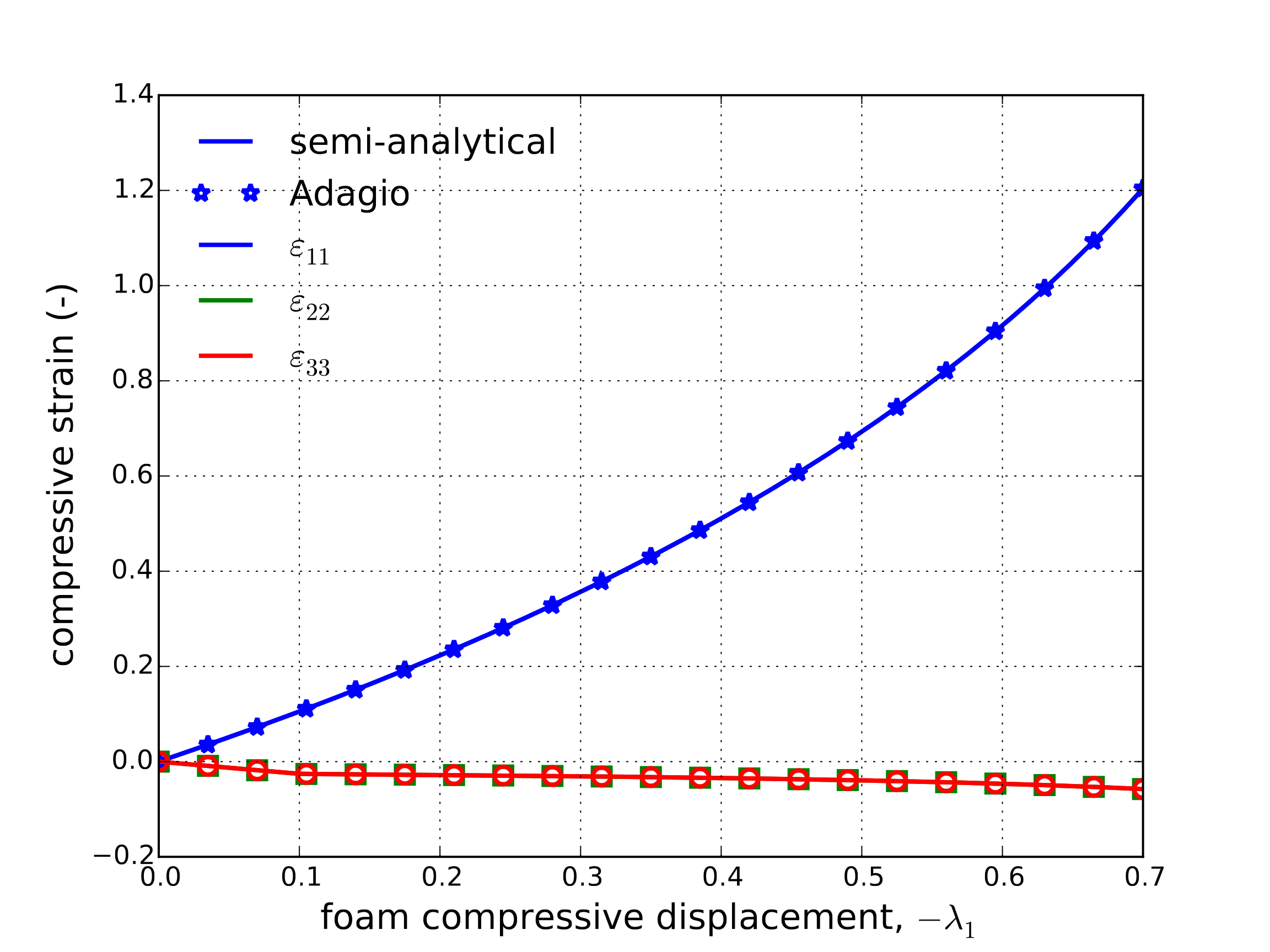
Fig. 4.127 Diagon strain evolution through a uniaxial displacement loading of the foam damage model considering (a) associated (\(\beta=0\)) and (b) radial (\(\beta=1\)) flow determined semi-analytically and numerically.

Specifically, in the radial case, only small off-axis strains are observed while in the associated results much more substantial strains are noted. This difference produces a large impact on the plastic volumetric strain and therefore on the maximum solid volume fraction, \(\phi\), whose evolution through loading in both cases is presented in Fig. 4.127. To emphasize this point, the radial solid volume fraction is more than double the associated case at the end of loading.

4.29.3.2. Uniaxial Tension

As the compressive and tensile behaviors of the model are different (due to the activation of the damage mechanism), the uniaxial tensile response is also investigated. To this end, a uniaxial displacement is applied, \(u_1=\lambda_1\), while the other off-axis components are kept traction free. For this test, the maximum displacement (\(\lambda_1=0.2\)) is applied linearly from \(t=0.0\) to \(t=1.0\). Use of a displacement condition is essential due to the expected stress degradation. In this case, given the relative values of the strength (\(a\left(\phi_0\right)\) versus \(c\)) it is clear that no plastic deformations will take place and a purely damage driven response is expected. With this simplification, it is also noted that the rate-dependency of the problem is eliminated. As the stress state is uniaxial, it is clear that the only non-zero eigenvalue of the stress tensor is \(\sigma_{11}\) and that \(\varepsilon_{\text{dam}}=a_{\text{dam}}\varepsilon_{11}=a_{\text{dam}}\ln\left(1+\lambda_1\right)\) where the fact that the plastic strain is zero is utilized. Bearing these simplifications in mind, an analytical expression for the stress and strain may be developed. The stress in the axial direction may be written as,

\[\begin{split}\sigma_{11}=\left\{\begin{array}{cc} \left(\mathbb{C}_{1111}-2\nu\mathbb{C}_{1122}\right)\ln\left(1+\lambda_1\right), & \lambda_1 < \lambda_{\text{crit}} \\ c\left(1-\frac{10}{3}a_{\text{dam}}\ln\left(1+\lambda_1\right)\right), & \lambda_1 \geq \lambda_{\text{crit}}\end{array} \right. ,\end{split}\]

where

\[\lambda_{\text{crit}}=\exp\left(\frac{c}{\mathbb{C}_{1111}-2\nu\mathbb{C}_{1122}+\frac{10}{3}a_{\text{dam}}c}\right)-1.\]

The analytical results along with numerical simulations from adagio are given below in Fig. 4.128.

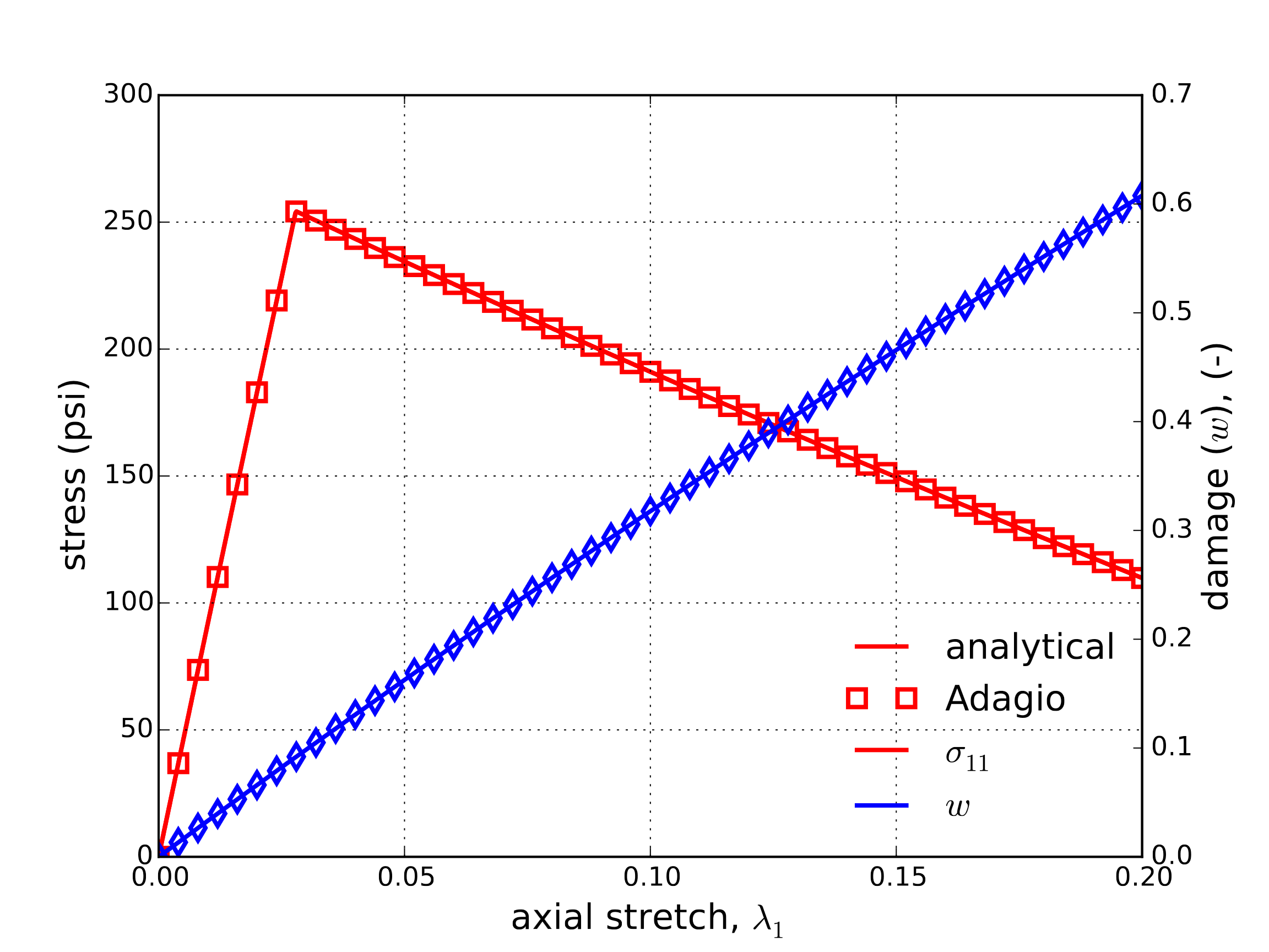
Fig. 4.128 Response of the foam damage model through a uniaxial stress, displacement controlled tension simulation. Stress in the loading direction, \(\sigma_{11}\), and damage measure, \(w\), against the applied displacement, \(\lambda_1\), are shown.

4.29.3.3. Hydrostatic Compression

To consider the pressure dependence, the response of this model subject to a hydrostatic compression loading is determined. Specifically, a displacement of the form \(u_i=\lambda\left(t\right)\) is considered. The applied displacement scales linearly from \(\lambda=0\) at \(t=0.0\) to \(\lambda=-0.7\) at \(t=t_{\text{max}}\). Two cases are considered to incorporate rate-dependent effects into the analysis. The two tests are denoted fast and slow and are distinguished via \(t_{\text{max}}\) values of 1.0 and 100.0, respectively. With this displacement field the engineering volume strain, \(\varepsilon_{\text{V}}\), is simply \(\varepsilon_{\text{V}}=\left(1+\lambda\right)^3-1\). The stress state reduces trivially to \(\sigma_{ij} = -p\delta_{ij}\) and the corresponding (repeated) eigenvalue is compressive. Therefore, damage does not play a role in this analysis.

No direct analytical solution to this problem is readily obtainable. Therefore, a semi-analytical analysis is used. Reducing the foam damage model for the loading described in this section leads to an expression for the overstess of,

\[\sigma^{*}=\frac{a}{b}|p|,\]

where the fact that \(s_{ij}=0\) is leveraged. Additionally, given this stress state, \(\beta\) becomes an unnecessary parameter as,

\[g_{ij}=g_{ij}^{\text{a}}=g_{ij}^{\text{r}}=-\frac{1}{\sqrt{3}}\text{sgn}\left(p\right)\delta_{ij},\]

with \(\text{sgn}\left(p\right)\) being the sign of \(p\). Both the numerical (adagio) and semi-analytical (evaluated in a forward Euler fashion) results are presented in Fig. 4.129.

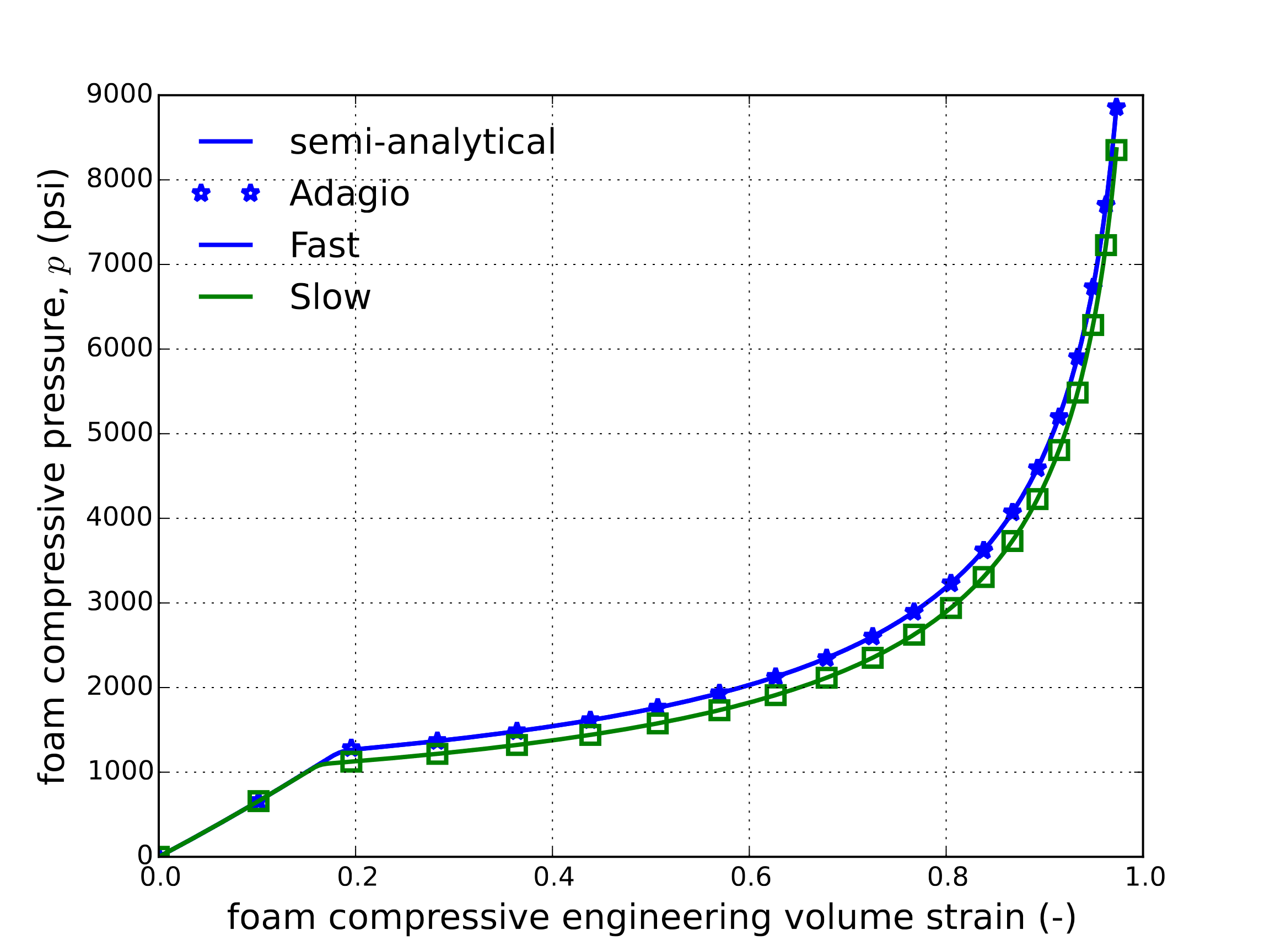
Fig. 4.129 Pressure-engineering volume strain results of the foam damage model subjected to a hydrostatic loading at both fast and slow rates determined semi-analytically and numerically.

4.29.3.4. Hydrostatic Tension

A tensile hydrostatic loading provides an interesting possibility for investigating the damage response. Specifically, with the model parameters defined above the damage tensile strength is always less than the hydrostatic strength - \(c < b\left(\phi_0\right)\). Additionally, given the tensile loading \(\phi\left(t\right)=\phi_0\) and no plastic deformation occurs. This also removes the rate-dependency form the model enabling an analytical solution to be obtained.

Through a hydrostatic loading, the only stress eigenvalue is \(-p\) (noting the convention of \(p\) positive in compression) and the corresponding strain eigenvalue is \(\varepsilon_{\text{max}}=\ln\left(1+\lambda\right)\). As no plastic deformation is occurring, the damage is simply a function of the deformation and is given by,

\[w\left(\varepsilon_{\text{dam}}\right)=w\left(\lambda\right)=\frac{10}{3}a_{\text{dam}}\ln\left(1+\lambda\right).\]

The pressure is then simply given as,

\[\begin{split}p=\left\{\begin{array}{cc} 3K\ln\left(1+\lambda\right) & \lambda < \lambda_{\text{crit}} \\ c\left(1-\frac{10}{3}a\ln\left(1+\lambda\right)\right) & \lambda \geq \lambda_{\text{crit}} \end{array} \right.,\end{split}\]

where,

\[\lambda_{\text{crit}}=\exp\left(\frac{3c}{9K+10c}\right)-1.\]

In the preceding relations, the fact that \(\varepsilon_{\text{dam}}=a\varepsilon_{\text{max}}\) is used. The analytical and numerical results are given below for a loading of \(\lambda=0\) to \(\lambda=0.2\) through the time period \(t=\left[0,1\right]\) in Fig. 4.130.

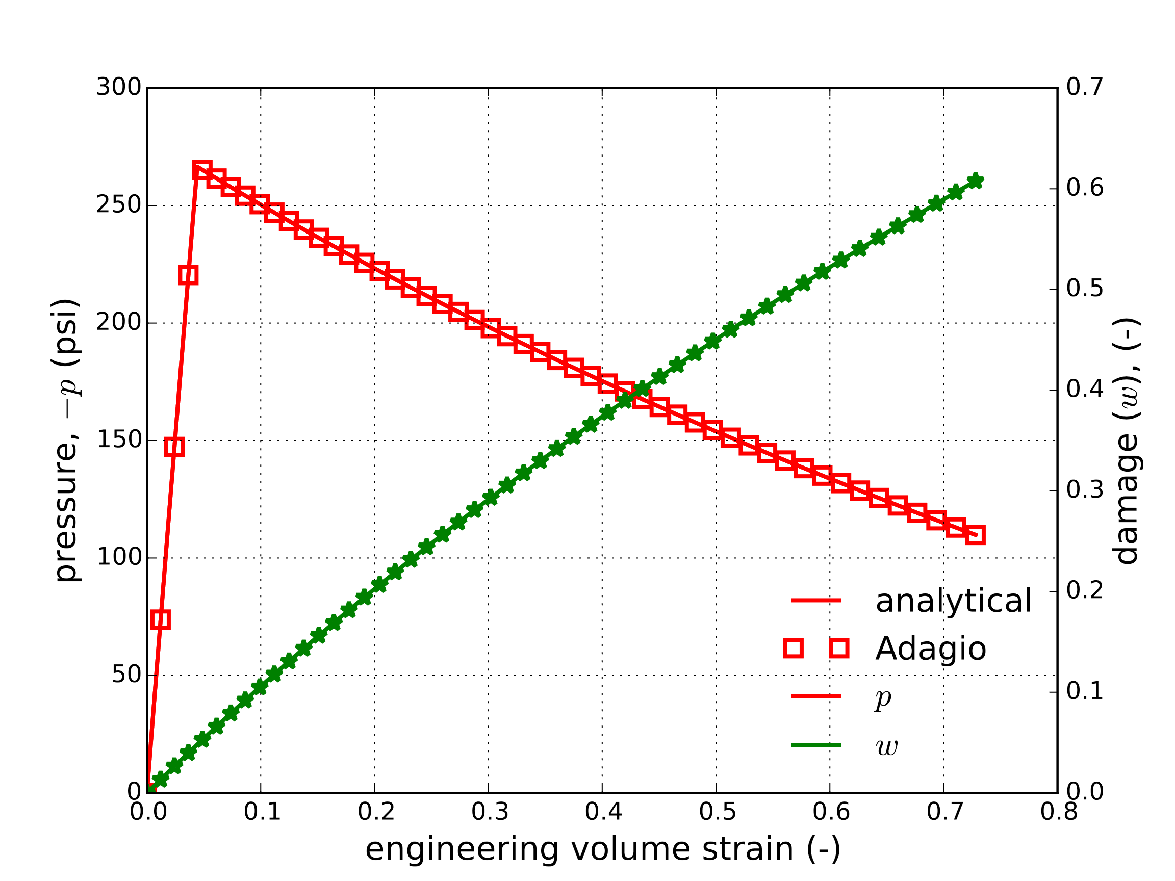
Fig. 4.130 Pressure and damage evolutions as function of engineering volume strain results of the foam damage model subject to a tensile hydrostatic loading determined analytically and numerically. Note, conventionally with this model pressure is defined positive in compression.

4.29.4. User Guide

BEGIN PARAMETERS FOR MODEL FOAM_DAMAGE
  #
  # Elastic constants
  #
  YOUNGS MODULUS = <real>
  POISSONS RATIO = <real>
  SHEAR MODULUS  = <real>
  BULK MODULUS   = <real>
  LAMBDA         = <real>
  TWO MU         = <real>
  #
  # Yield behavior
  #
  PHI               = <real>
  FLOW RATE         = <real>
  POWER EXPONENT    = <real>
  TENSILE STRENGTH  = <real>
  ADAM              = <real>
  BDAM              = <real>
  #
  # Functions
  #
  YOUNGS FUNCTION          = <string>
  POISSONS FUNCTION        = <string>
  RATE FUNCTION            = <string>
  EXPONENT FUNCTION        = <string>
  SHEAR HARDENING FUNCTION = <string>
  HYDRO HARDENING FUNCTION = <string>
  BETA FUNCTION            = <string>
  YOUNGS PHI FUNCTION      = <string>
  POISSONS PHI FUNCTION    = <string>
  DAMAGE FUNCTION          = <string>
END [PARAMETERS FOR FOAM_DAMAGE]

Output variables available for this model are listed in Table 4.46. For information about the foam damage model, consult [[1]].

Table 4.46 State Variables for FOAM DAMAGE Model

Name	Description
ITER	number of sub-increments taken in subroutine
EPVOL	plastic volume strain
PHI	maximum volume fraction of solid material
EQPS	equivalent plastic strain
FA	shear strength - \(a\)
FB	hydrostatic strength - \(b\)
DAMAGE	damage
EMAX	maximum tensile strain
PWORK	plastic work rate

---

[1] (1,2,3)

M. K. Neilsen, W. Y. Lu, W. M. Scherzinger, T. D. Hinnerichs, and C. S. Lo. Unified creep plasticity damage (UCPD) model for rigid polyurethane foams. Technical Report SAND2015-4352, Sandia National Laboratories, Albuquerque, NM, 2015.