4.8. Elastic-Plastic Power Law Hardening Model

4.8.1. Theory

The elastic-plastic power law hardening model is a hypoelastic, rate-independent plasticity model with power law hardening [[1]]. The rate form of the constitutive equation assumes an additive split of the rate of deformation into an elastic and plastic part

\[D_{ij} = D^{\text{e}}_{ij} + D^{\text{p}}_{ij}\]

The stress rate only depends on the elastic strain rate in the problem

\[\stackrel{\circ}{\sigma}_{ij} = \mathbb{C}_{ijkl}D^{\text{e}}_{kl}\]

where \(\mathbb{C}_{ijkl}\) are the components of the fourth-order, isotropic elasticity tensor.

The key to integrating the model is finding the plastic rate of deformation. For associated flow the plastic rate of deformation is in a direction normal to the yield surface. The yield surface is given by

(4.33)\[f\left( \sigma_{ij},\bar{\varepsilon}^{p} \right) = \phi\left(\sigma_{ij}\right) - \bar{\sigma} \left( \bar{\varepsilon}^{p} \right) = 0\]

where \(\phi\) is the equivalent stress and \(\bar{\sigma}\) is the hardening function which is a function of the equivalent plastic strain \(\bar{\varepsilon}^{p}\). For this model the hardening function uses a power law

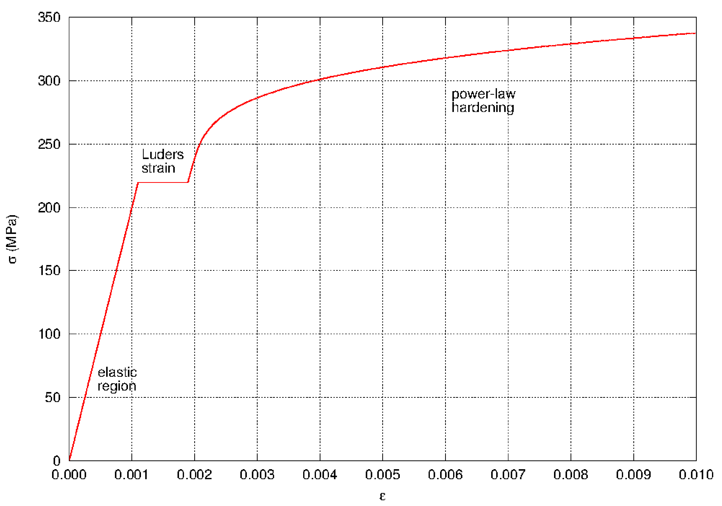
Fig. 4.20 Typical stress-strain response for the power-law hardening model.

\[\bar{\sigma} \left( \bar{\varepsilon}^{p} \right) = \sigma_{y} + A \left< \bar{\varepsilon}^{p} -\varepsilon_{L} \right>^{n}\]

which is shown in Fig. 4.20. The yield stress is \(\sigma_{y}\), the hardening constant is \(A\), the hardening exponent is \(n\), and the L"{u}ders strain is \(\varepsilon_{L}\). The bracket \(<\cdot>\) is the Macaulay bracket defined as

\[\begin{split}\left< x \right> = \begin{cases} 0,& \text{if } x \leq 0\\ x,& \text{if } x > 0. \end{cases}\end{split}\]

By assuming associated plastic flow, the plastic rate of deformation can be written as

(4.34)\[D^{\text{p}}_{ij} = \dot{\gamma}\frac{\partial\phi}{\partial\sigma_{ij}}.\]

For this model the yield surface is chosen to be a von Mises yield surface, so

\[\phi\left(\sigma_{ij}\right) = \sqrt{\frac{3}{2}s_{ij}s_{ij}}\]

where \(s_{ij}\) are the components of the deviatoric stress

\[s_{ij} = \sigma_{ij} - \frac{1}{3}\delta_{ij}\sigma_{kk}\]

Unlike the elastic-plastic model Section 4.7, the power-law hardening model does not allow for kinematic hardening, so there is no back stress.

4.8.2. Implementation

The elastic-plastic power-law hardening model is implemented using a predictor-corrector algorithm. First, an elastic trial stress state is calculated. This is done by assuming that the rate of deformation is completely elastic

\[ T^{tr}_{ij} = T^{n}_{ij} + \Delta t \left( \lambda\delta_{ij}d_{kk} + 2\mu d_{ij} \right)\]

The trial stress state is decomposed into a pressure and a deviatoric stress

\[ p^{tr} = \frac{1}{3} T^{tr}_{kk} \;\;\; ; \;\;\; s^{tr}_{ij} = T^{tr}_{ij} - p^{tr}\delta_{ij}\]

The effective trial stress is calculated and and used in the yield function~eqref{eq:EPyield}.

\[f \left( s^{tr}_{ij},\bar{\varepsilon}^{p} \right) = \phi \left( s^{tr}_{ij} \right) - \bar{\sigma}\left( \bar{\varepsilon}^{p} \right)\]

If \(f \leq 0\) then the strain rate is elastic and the stress update is finished. If \(f > 0\) then plastic deformation has occurred and a radial return algorithm determines the extent of plastic deformation.

The normal to the yield surface is assumed to lie in the direction of the trial stress state. This gives us the following expression for \(N_{ij}\)

\[N_{ij} = \frac{s_{ij}^{tr}}{\|s_{ij}^{tr}\|}\]

Using a backward Euler algorithm, the final deviatoric stress state is

\[s^{n+1}_{ij} = s_{ij}^{tr} - \Delta \, t 2\mu d_{ij}^{\text{p}}\]

where the plastic strain increment is

\[\Delta d_{ij}^{\text{p}} = \sqrt{\frac{3}{2}} \Delta\bar{\varepsilon}^{p} N_{ij}\]

The equation for the change in the equivalent plastic strain over the load step is found as the solution to

\[3 \mu \Delta\bar{\varepsilon}^{p} + \bar{\sigma}\left( \bar{\varepsilon}_{n} + \Delta\bar{\varepsilon}^{p} \right) - \phi^{tr} + f_{n} = 0\]

4.8.3. Verification

The elastic-plastic power-law hardening model is verified for uniaxial stress and pure shear. The elastic properties used in these analyses are \(E = 70\) GPa and \(\nu = 0.25\). The hardening law used for the model is

\[\bar{\sigma}\left(\bar{\varepsilon}^{p}\right) = \sigma_{y} + A \left< \bar{\varepsilon}^{p} - \varepsilon_{L} \right>^{n}\]

For these calculations \(\sigma_{y} = 200\) MPa, \(A = 400\) MPa, \(n = 0.25\), and \(\varepsilon_{L} = 0.008\).

4.8.3.1. Uniaxial Stress

The elastic-plastic power-law hardening model is tested in uniaxial tension. The test looks at the axial stress and the lateral strain and compares these values against analytical results for the same problem. In this verification problem only the normal strains/stresses are needed, and the shear terms are not exercised.

For the uniaxial stress problem, the only non-zero stress component is \(\sigma_{11}\). In the analysis that follows \(\sigma_{11} = \sigma\). There are three non-zero strain components, \(\varepsilon_{11}\), \(\varepsilon_{22}\), and \(\varepsilon_{33}\). In the analysis that follows \(\varepsilon_{11} = \varepsilon\) and \(\varepsilon_{22} = \varepsilon_{33}\). Furthermore, the axial elastic strain, \(\varepsilon_{11}^{\text{e}} = \sigma/E\) will be denoted by \(\varepsilon^{\text{e}}\).

The equivalent plastic strain, \(\bar{\varepsilon}^{\text{p}}\), for this model is equivalent to \(\varepsilon_{11}^{\text{p}}\), and is

\[\bar{\varepsilon}^{\text{p}} = \varepsilon - \frac{\bar{\sigma}\left(\bar{\varepsilon}^{\text{p}}\right)}{E}\]

This allows us, after yield, to parameterize the problem with the equivalent plastic strain.

For the lateral strains we need the lateral plastic strain. Plastic incompressibility (\(\varepsilon^{\text{p}}_{kk}=0\)) gives us

\[\varepsilon^{\text{p}}_{22} = -\frac{1}{2}\bar{\varepsilon}^{\text{p}}\]

Combined with the lateral elastic strains we have the lateral strain as a function of the equivalent plastic strain

\[\varepsilon_{22} = -\nu\frac{\bar{\sigma}\left(\bar{\varepsilon}^{\text{p}}\right)}{E} - \frac{1}{2}\bar{\varepsilon}^{\text{p}}\]

The results are shown in Fig. 4.21 and Fig. 4.22 and show agreement between the model in Adagio and the analytical results.

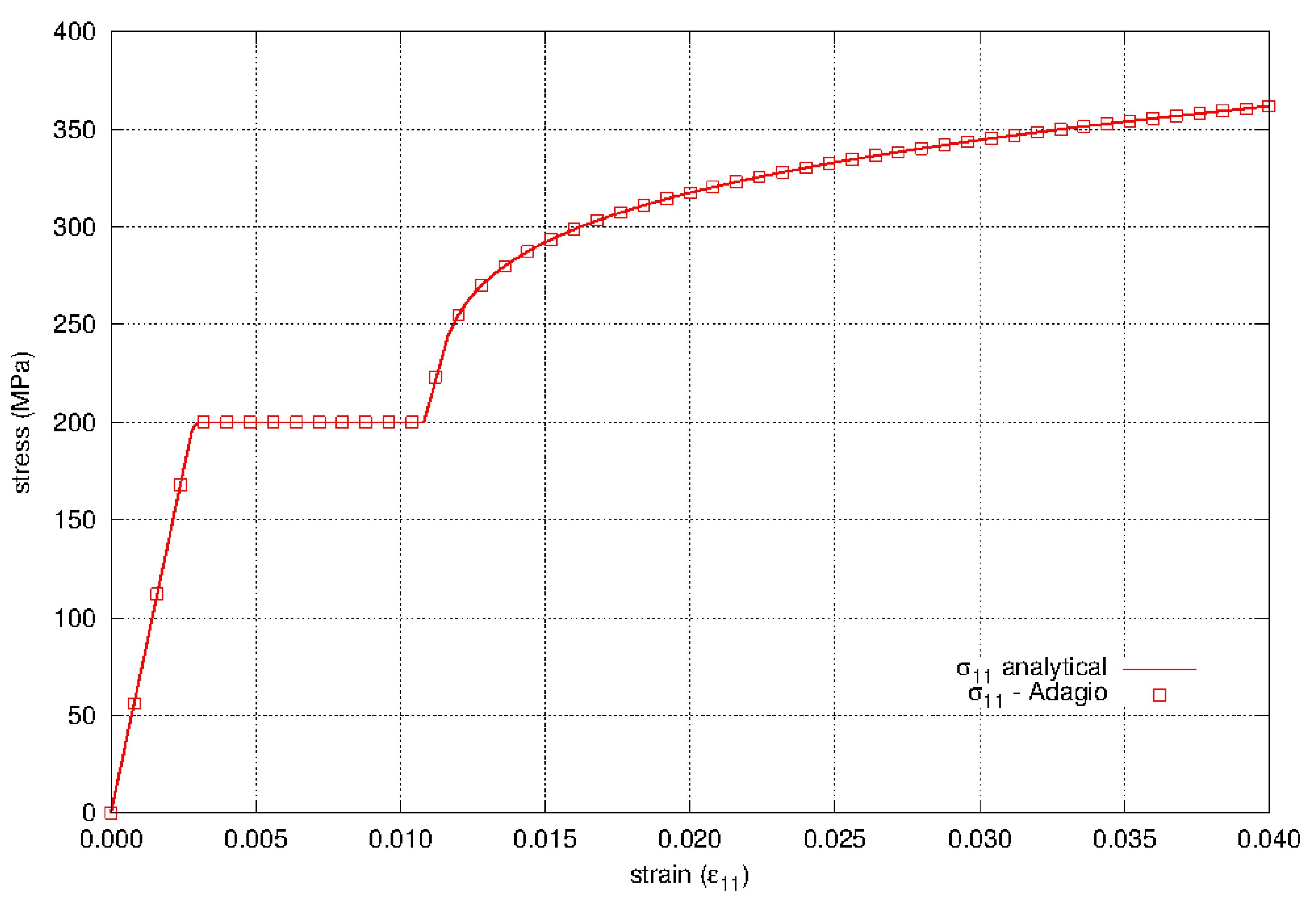
Fig. 4.21 The axial stress as a function of axial strain for the elastic-plastic power-law hardening model.

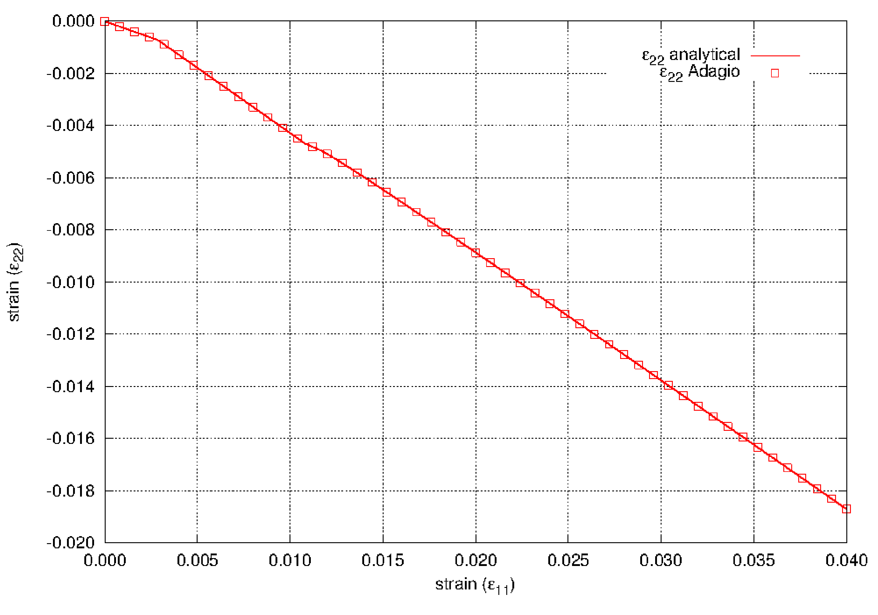
Fig. 4.22 The lateral strain as a function of axial strain for the elastic-plastic power-law hardening model.

4.8.3.2. Pure Shear

The elastic-plastic power-law hardening model is tested in pure shear. The test looks at the shear stress as a function of the shear strain and compares these values against analytical results for the same problem. For the pure shear problem, the only non-zero strain component is \(\varepsilon_{12}\) and the only non-zero stress component is \(\sigma_{12}\).

After yield, the shear stress as a function of the hardening curve is \(\sigma_{12} = \bar{\sigma}\left(\bar{\varepsilon}^{\text{p}}\right)/\sqrt{3}\). The elastic shear strain is \(\varepsilon_{12}^{\text{e}} = \sigma_{12}/2G\); the plastic shear strain is \(\varepsilon_{12}^{\text{p}} = \sqrt{3}\bar{\varepsilon}^{\text{p}}/2\). Using this, the shear stress and strain are given as functions of the equivalent plastic strain

\[\sigma_{12} = \frac{\bar{\sigma}\left(\bar{\varepsilon}^{\text{p}}\right)}{\sqrt{3}} \;\;\; ; \;\;\; \varepsilon_{12} = \frac{\sqrt{3}}{2} \bar{\varepsilon}^{\text{p}} + \frac{1}{\sqrt{3}}\frac{\bar{\sigma}\left(\bar{\varepsilon}^{\text{p}}\right)}{2\mu}\]

This allows us, after yield, to parameterize the problem with \(\bar{\varepsilon}^{\text{p}}\).

The results are shown in Fig. 4.23 and show agreement between the model in Adagio and the analytical results.

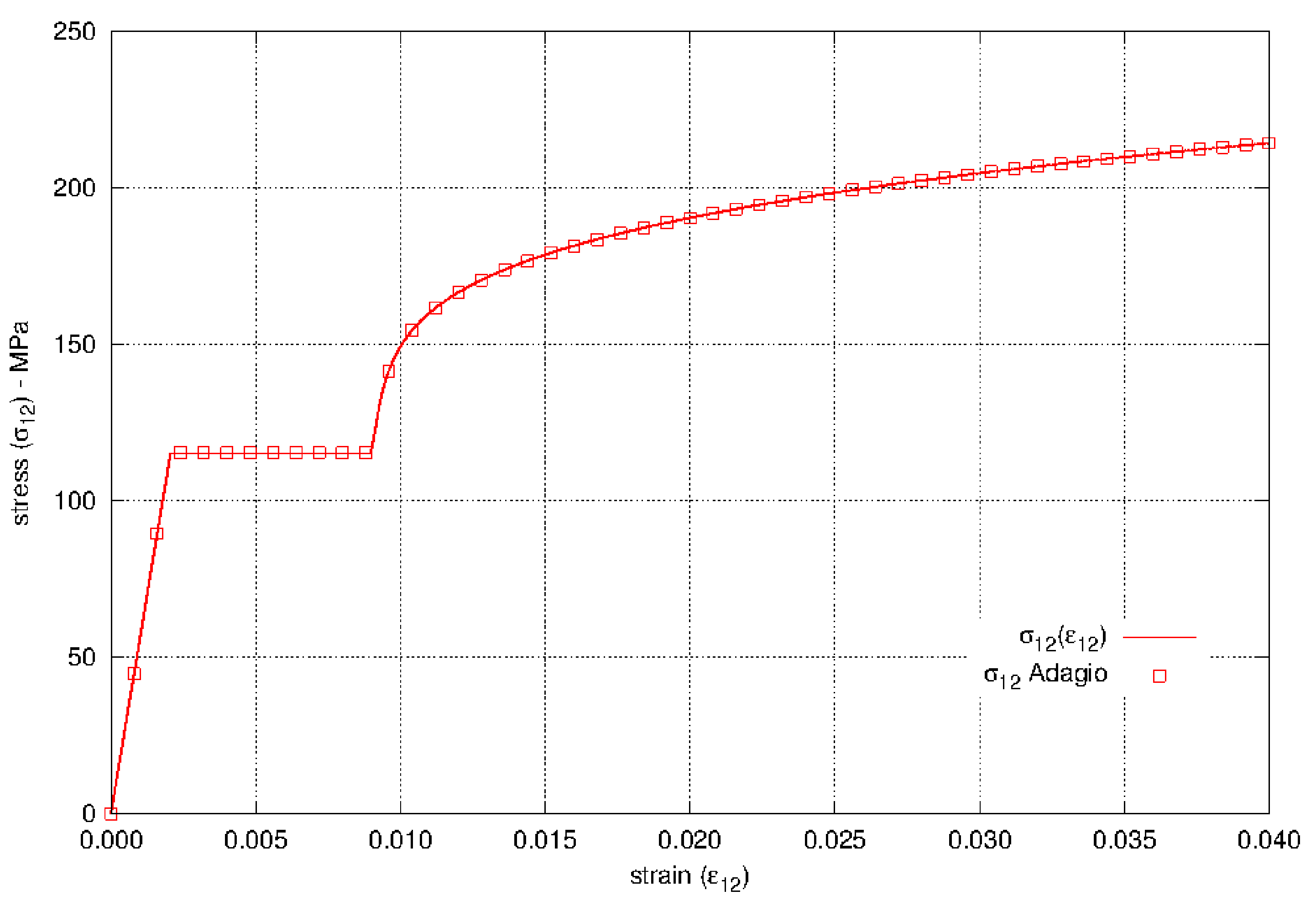
Fig. 4.23 The shear stress as a function of shear strain for the elastic-plastic power-law hardening model.

4.8.4. User Guide

BEGIN PARAMETERS FOR MODEL EP_POWER_HARD
  #
  # Elastic constants
  #
  YOUNGS MODULUS = <real>
  POISSONS RATIO = <real>
  SHEAR MODULUS  = <real>
  BULK MODULUS   = <real>
  LAMBDA         = <real>
  TWO MU         = <real>
  #
  # Hardening behavior
  #
  YIELD STRESS       = <real>
  HARDENING CONSTANT = <real>
  HARDENING EXPONENT = <real>
  LUDERS STRAIN      = <real>
END [PARAMETERS FOR MODEL EP_POWER_HARD]

In the above command blocks:

• The YIELD STRESS is the stress at which the plastic power law yielding and hardening model takes effect. See Fig. 4.20.

• The LUDERS STRAIN defines a regime of zero hardening modulus prior to onset of the power law hardening. A small Luder band is seen in the hardening behavior or many metals. See Fig. 4.20 for details.

• The HARDENING CONSTANT command line and HARDENING EXPONENT command define the power law hardening curve. Past the Luder strain the hardened yield surface radius is given by the HARDENING CONSTANT times plastic strain to the HARDENING EXPONENT power.

Output variables available for this model are listed in Table 4.7 and Table 4.8. For information about the elastic-plastic power-law hardening model, consult [[2]].

Table 4.7 State Variables for EP POWER HARD Model

Name	Description
EQPS	equivalent plastic strain, \(\bar{\varepsilon}^{p}\)
TENSILE_EQPS	equivalent plastic strain only accumulated when the material is in tension (trace of stress tensor is positive)
RADIUS	radius of yield surface, \(R\)
ITERATIONS	number of radial return iterations

Table 4.8 State Variables for EP POWER HARD Model for Shells

Name	Description
EQPS	equivalent plastic strain, \(\bar{\varepsilon}^{p}\)
TENSILE_EQPS	equivalent plastic strain only accumulated when the material is in tension (trace of stress tensor is positive)
RADIUS	radius of yield surface, \(R\)
ITERATIONS	number of radial return iterations
ERROR	error in plane stress iterations
PS_ITER	plane stress iterations

---

[1]

C. M. Stone, G. W. Wellman, and R. D. Krieg. A vectorized elastic/plastic power law hardening material model including Lüders strains. Technical Report SAND90-0153, Sandia National Laboratories, Albuquerque, NM, March 1990. \href http://infoserve.sandia.gov/sand_doc/1990/900153.pdfpdf.

[2]

C.M. Stone. SANTOS – a two-dimensional finite element program for the quasistatic, large deformation, inelastic response of solids. Technical Report SAND90-0543, Sandia National Laboratories, Albuquerque, NM, 1996. \href http://infoserve.sandia.gov/sand_doc/1990/900543.pdfpdf.