4.9. Ductile Fracture Model

4.9.1. Theory

The ductile fracture model is identical to the elastic-plastic power-law hardening model with the addition of a failure criterion and an isotropic decay of the stress to zero during the failure process within the constitutive model. To accomplish this task, the tearing parameter, \(t_p\), proposed by Wellman [[1]] is introduced and the functional form as given as

(4.35)\[t_{p} = \int_0^{\varepsilon} {\Big\langle \frac{{2\sigma_{\max}}}{{3\left( {\sigma_{\max} - \sigma_{m} } \right)}}\Big\rangle } ^4 d\bar{\varepsilon}^{p}\]

where \(\sigma_{\max }\) is the maximum principal stress, and \(\sigma _{m}\) is the mean stress. It can also be noted that the tearing parameter evolves during the plastic deformation regime as indicated by integrating over the effective plastic strain, \(\bar{\varepsilon}^{p}\). The angle brackets denoting the Macaulay brackets, where

\[\begin{split}\langle x \rangle = \begin{cases} 0 \;\;\; \text{if } x \leq 0 \\ x \;\;\; \text{if } x > 0 \end{cases},\end{split}\]

are used to ensure that the failure process occurs only with tensile stress states and prevent “damage healing”. The failure process then initiates at a critical tearing parameter, \(t_p^{\text{crit}}\), and the corresponding stress decay occurs over a strain interval corresponding to the critical crack opening strain, \(\varepsilon_{\text{ccos}}\). Importantly, the \(\varepsilon_{\text{ccos}}\) serves a dual role in that it may also be used to control the energy dissipated during failure. With respect to the latter point, careful selection of the critical crack opening strain may be used to ensure consistent energy is dissipated through different meshes. This decay process is isotropic and linear with the current damage value being equivalent to the ratio of crack opening strain in the direction of the maximum principal stress to the critical value.

4.9.2. Implementation

The ductile fracture model seeks to capture both the nonlinear elastic-plastic and fracture responses of a ductile metal. Independently, each of these requirements necessitates the use of a nonlinear solution algorithm and the combination of the two is even more complex. This consideration is compounded by the relaxation and softening observed during the failure process that introduces additional complications for the global finite element solver. For this discussion, however, the focus is solely on the underlying numerical treatment of the failure process at the constitutive level. The solution of the elastic-plastic constitutive problem was discussed in detail in Section 4.8.2 while details of the implications at the global finite element problem are found in the Sierra/SM User’s Manual [[2]]. With respect to the latter, it is important to note that in quasistatic cases the ductile fracture model is tightly integrated with the multilevel CONTROL FAILURE capabilities although details of this coupling are left to [[1], [2]].

Prior to fracture initiation – while \(t_p^{n+1}<t_p^{\text{crit}}\) – the ductile fracture model is exactly that of the elastic-plastic power law. Through this process the tearing parameter is continually calculated at the plastically converged state. When fracture initiation is first detected – \(t_p^{n+1}\geq t_p^{\text{crit}}\) – the direction of the maximum principal stress, denoted by the normalized vector \(n^{cr}_i\), is determined and stored. Regardless of loading path, this vector does not change during the unloading process. Additionally, for this first initial failure step, the unrotated stress tensor, \(T_{ij}\) must be set equal to its maximum value, \(T^{\text{crit}}_{ij}\) before any unloading may be performed. This maximum value is simply given by,

\[T^{\text{crit}}_{ij}=T^n_{ij}+\left(T^{tr}_{ij}-T_{ij}^n\right)\frac{t_p^{\text{crit}}-t_p^n}{t_p^{n+1}-t_p^n}\]

with \(T_{ij}^{tr}\) being the elastic trial stress. As alluded to in the prior section, a linear decay based on the crack opening strain in the direction of maximum stress, \(\varepsilon_{\text{cos}}\), is utilized. To determine this decay value, the crack opening strain increment is first found via

\[d\varepsilon^{n+1}_{\text{cos}}=<\beta n^{cr}_id^{n+1}_{ij}n^{cr}_j>,\]

where \(d^{n+1}_{ij}\) is the total unrotated rate of deformation and \(\beta\) is a partitioning factor between plastic and crack opening strains and takes the value of 1 for all loading steps emph{except} the initiation step. The \(<\cdot>\) are the Macaulay brackets. During the first fracture step,

\[\beta=\frac{t_p^{n+1}-t_p^{\text{crit}}}{t_p^{n+1}-t_p^n}.\]

The current crack opening strain is then simply,

\[\varepsilon^{n+1}_{\text{cos}}=\varepsilon^n_{\text{cos}}+d\varepsilon^{n+1}_{\text{cos}}\Delta t\]

and the decay value, \(\alpha^{n+1}\), is then found as,

\[\alpha^{n+1}=\max\left[0,\frac{\varepsilon_{\text{ccos}}-\varepsilon^{n+1}_{\text{cos}}}{\varepsilon_{\text{ccos}}}\right].\]

To perform the actual stress decay, the hardening and yield values are proportionally decayed via,

\[\bar{\sigma}^{n+1}\left(\bar{\varepsilon}^p\right)=\alpha^{n+1}\bar{\sigma}^f;\qquad\beta_{ij}^{n+1}=\alpha^{n+1}\beta_{ij}^n,\]

with \(\bar{\sigma}^f=\phi\left(T^{\text{crit}}_{ij}\right)\) being the critical yield stress associated with the yield surface, \(\phi\), and \(\beta_{ij}\) is the backstress tensor used with kinematic hardening. The decayed stress is then found by radially returning to the reduced yield stress, \(\bar{\sigma}^{n+1}\left(\bar{\varepsilon}\right)\). As a \(J_2\) deviatoric yield stress is used for the plastic response, the hydrostatic component of the stress tensor is similarly decayed.

4.9.3. Verification

The ductile fracture model is tested in uniaxial stress and pure shear. For these test problems, the Young’s modulus and Poisson’s ratio are \(E = 70\) GPa and \(\nu = 0.25\). The yield stress is taken to be \(\sigma_y = 200\) MPa while the hardening constant and exponent are \(A=400\) MPa and \(n = 0.25\), respectively, and the Luders strain is \(0.008\). To describe failure, the critical tearing parameter is \(t_{p}^{\text{crit}} = 0.025\) and the critical crack opening strain is \(\varepsilon_{\text{ccos}} = 0.001\).

4.9.3.1. Uniaxial Stress

For loading in uniaxial stress the only non-zero stress component is \(\sigma_{11}\). All other stress components are zero. If the stress state is on the yield surface then this stress is

\[\sigma_{11} = \bar{\sigma}(\bar{\varepsilon}^{p}),\]

with \(\bar{\sigma}\) being the yield stress including any hardening effects associated with the evolution of the effective plastic strain, \(\bar{\varepsilon}^p\). To evaluate the axial stress we need the equivalent plastic strain as a function of the axial strain, \(\varepsilon_{11}\). If we equate the rate of plastic work we get

\[\bar{\sigma}\dot{\bar{\varepsilon}}^{p} = \sigma_{11} \left( \dot{\varepsilon}_{11} - \dot{\varepsilon}_{11}^{\text{e}} \right) \;\;\; \rightarrow \;\;\; \dot{\bar{\varepsilon}}^{p} = \dot{\varepsilon}_{11} - \dot{\varepsilon}_{11}^{\text{e}} = \dot{\varepsilon}^p_{11}\]

which, when integrated, gives us an implicit equation for the equivalent plastic strain

\[\bar{\varepsilon}^{p} = \left( \varepsilon_{11} - \frac{\bar{\sigma}(\bar{\varepsilon}^{p})}{E} \right).\]

Alternatively, we write the axial strain as a function of the equivalent plastic strain, which allows us to parameterize the problem with \(\bar{\varepsilon}^{p}\)

\[\varepsilon_{11} = \bar{\varepsilon}^{p} + \frac{\bar{\sigma}(\bar{\varepsilon}^{p})}{E}.\]

In uniaxial stress the pressure is \(\sigma_{11}/3\) and the maximum principal stress is \(\sigma_{\text{max}} = \sigma_{11}\). Using this in (4.35) we get

\[t_{p} = \bar{\varepsilon}^{p}\]

i.e. the tearing parameter is equal to the equivalent plastic strain. This result is shown in Fig. 4.24(a). The final value for the tearing parameter is a function of the number of steps, or the step size. The smaller the step size the closer the final value is to \(t_{p}^{\text{crit}}\).

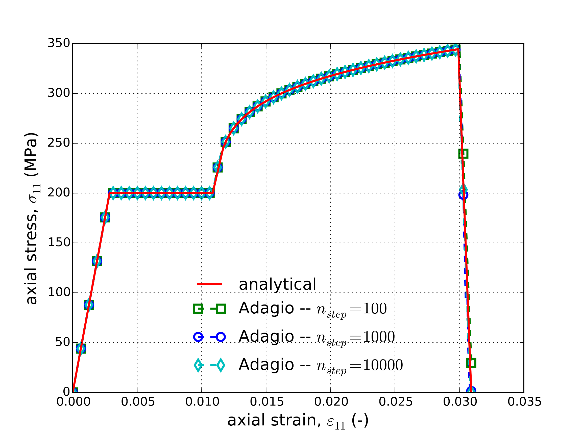
The axial stress as a function of axial strain is shown in Fig. 4.24(b). The axial stress depends on the elastic-plastic response until the critical tearing parameter is reached. As with the tearing parameter results, this point is time step dependent. Once the critical tearing parameter is reached the stress decay occurs over the critical crack opening strain.

Tearing parameter

Axial stress

Fig. 4.24 The (a) tearing parameter, \(t_{p}\), and (b) axial stress-strain response for the ductile fracture model in uniaxial stress. The post failure reduction in stress depends on the time discretization or step size.

4.9.3.2. Pure Shear

For loading in pure shear the only non-zero stress component is \(\sigma_{12}\). All other stress components are zero. If the stress state is on the yield surface then the shear stress is

\[\sigma_{12} = \frac{\bar{\sigma}(\bar{\varepsilon}^{p})}{\sqrt{3}}.\]

To evaluate the shear stress we need the equivalent plastic strain as a function of the shear strain. If we equate the rate of plastic work we get

\[\bar{\sigma}\dot{\bar{\varepsilon}}^{p} = 2\sigma_{12} \left( \dot{\varepsilon}_{12} - \dot{\varepsilon}_{12}^{\text{e}} \right) \;\;\; \rightarrow \;\;\; \dot{\bar{\varepsilon}}^{p} = \frac{2}{\sqrt{3}} \left( \dot{\varepsilon}_{12} - \dot{\varepsilon}_{12}^{\text{e}} \right)\]

which, when integrated, gives us an implicit equation for the equivalent plastic strain

\[\bar{\varepsilon}^{p} = \frac{2}{\sqrt{3}} \left( \varepsilon_{12} - \frac{\bar{\sigma}(\bar{\varepsilon}^{p})}{\sqrt{3}G} \right).\]

Alternatively, we write the shear strain, \(\varepsilon_{12}\) as a function of the equivalent plastic strain, which allows us to parameterize the problem with \(\bar{\varepsilon}^{p}\)

\[\varepsilon_{12} = \frac{\sqrt{3}}{2} \bar{\varepsilon}^{p} + \frac{\bar{\sigma}(\bar{\varepsilon}^{p})}{\sqrt{3}G}.\]

In pure shear the pressure is zero, and the maximum principal stress is \(\sigma_{\text{max}} = \sigma_{12}\). Using this in (4.35) we get

\[t_{p} = \left( \frac{2}{3} \right)^{4} \bar{\varepsilon}^{p}.\]

This result is shown in Fig. 4.25, where the tearing parameter is a function of the shear strain. The final value for the tearing parameter is a function of the number of steps, or the step size. The smaller the step size the closer the final value is to \(t_{p}^{\text{crit}}\).

The shear stress as a function of shear strain is shown in Fig. 4.26. The shear stress depends on the elastic-plastic response until the critical tearing parameter is reached. As with the tearing parameter results, this point is time step dependent. Once the critical tearing parameter is reached the stress decay occurs over the critical crack opening strain.

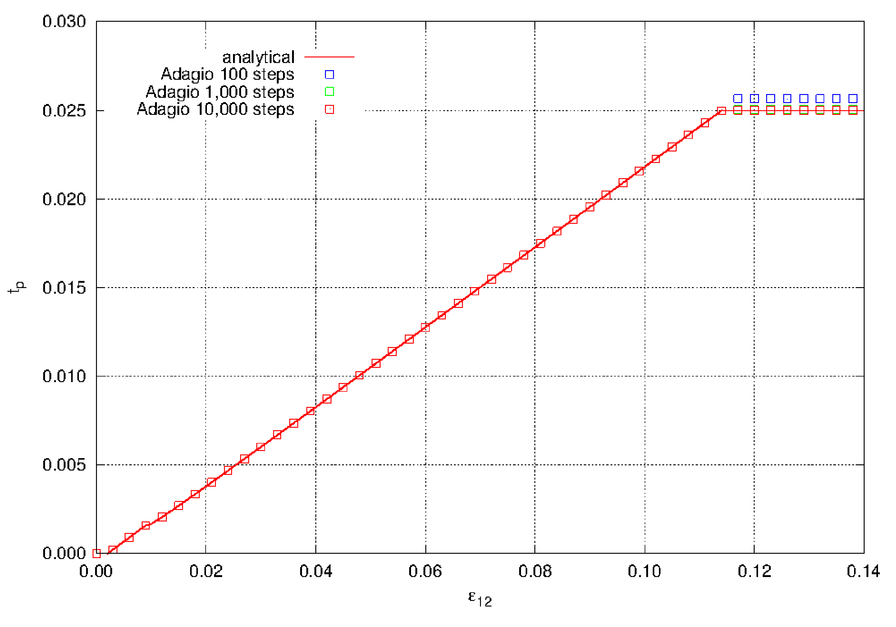
Fig. 4.25 The tearing parameter, \(t_{p}\), in pure shear. The maximum tearing parameter depends on the time discretization or step size.

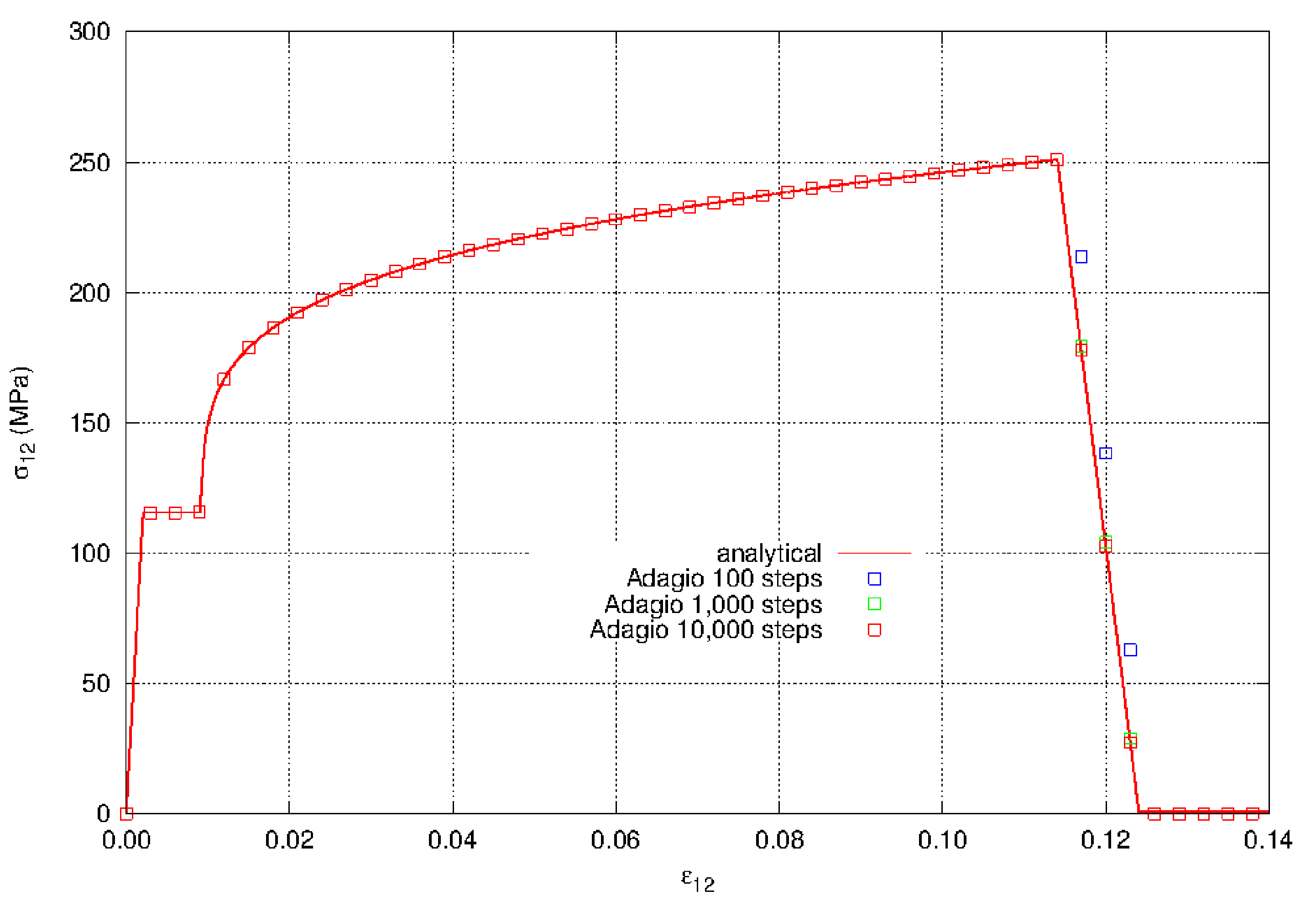
Fig. 4.26 Shear stress vs. shear strain for the ductile fracture model in pure shear. The post failure reduction in stress depends on the time discretization or step size.

4.9.4. User Guide

BEGIN PARAMETERS FOR MODEL DUCTILE_FRACTURE
  #
  # Elastic constants
  #
  YOUNGS MODULUS = <real>
  POISSONS RATIO = <real>
  SHEAR MODULUS  = <real>
  BULK MODULUS   = <real>
  LAMBDA         = <real>
  TWO MU         = <real>
  #
  # Yield surface parameters
  #
  YIELD STRESS       = <real>
  HARDENING CONSTANT = <real>
  HARDENING EXPONENT = <real>
  LUDERS STRAIN      = <real>
  #
  # Failure parameters
  #
  CRITICAL TEARING PARAMETER    = <real>
  CRITICAL CRACK OPENING STRAIN = <real>
END [PARAMETERS FOR MODEL DUCTILE_FRACTURE]

In the above command blocks:

• The YIELD STRESS is the stress at which the plastic power load yielding and hardening model takes effect. See Fig. 4.20.

• The LUDERS STRAIN defines a regime of zero hardening modulus prior to onset of the power law hardening. A small Luder band is seen in the hardening behavior or many metals. See Fig. 4.20 for details.

• The HARDENING CONSTANT command line and HARDENING EXPONENT command define the power law hardening curve. Past the Luder strain the hardened yield surface radius is given by the HARDENING CONSTANT times plastic strain to the HARDENING EXPONENT power.

• CRITICAL TEARING PARAMETER defines the \(t_{p}\) value at which fracture and subsequent decay of stress will occur.

• When the model undergoes additionally strain after reaching the critical tearing parameter the stress in the model will decay to zero. The amount strain over which the stress decays to zero is defined with the CRITICAL CRACK OPENING STRAIN command line. The relevant opening strain is the component of strain that is aligned with the maximum-principal-stress direction at initial failure.

Output variables available for this model are listed in Table 4.9. For information about the ductile fracture material model, consult [[1]].

Table 4.9 State Variables for DUCTILE FRACTURE Model

Name	Description
EQPS	equivalent plastic strain, \(\bar{\varepsilon}^{p}\)
RADIUS	radius of yield surface, \(R\)
BACK_STRESS	back stress - tensor \(\alpha_{ij}\)
TEARING_PARAMETER	Current value of the integrated tearing parameter
CRACK_OPENING_STRAIN	Current value of the crack opening strain. Will be zero prior to reaching the maximum tearing parameter.
FAILURE_DIRECTION	Crack opening direction (maximum principal stress direction at failure) - vector
DF_STRAIN_XX	XX component of current strain
DF_STRAIN_YY	YY component of current strain
DF_STRAIN_ZZ	ZZ component of current strain
DF_STRAIN_XY	XY component of current strain
DF_STRAIN_YZ	YZ component of current strain
DF_STRAIN_ZX	ZX component of current strain
MAX_RADIUS	Yield surface radius at failure
MAX_PRESS	Stress pressure norm at failure

---

[1] (1,2,3)

G. W. Wellman. A simple approach to modeling ductile failure. Technical Report SAND2012-1343, Sandia National Laboratories, Albuquerque, NM, June 2012. \href http://infoserve.sandia.gov/sand_doc/2012/121343.pdfpdf.

[2] (1,2)

Sierra/SolidMechanics Team. Sierra/SolidMechanics VOTD User’s Guide. Technical Report In draft, Sandia National Laboratories, Albuquerque, NM, 2019.