4.22. Hyperfoam Model

4.22.1. Theory

The hyperfoam model is a hyperelastic model that can be used for modeling elastomeric foams. It is based on a strain energy with a form given by Storakers [[1]] which is similar to a form presented by Ogden [[2]]. The strain energy depends on the principal stretch ratios of the material and is given by

(4.108)\[W(\lambda_{k}) = \sum_{i=1}^{N} \frac{2\mu_{i}}{\alpha_{i}^{2}} \left[ \lambda_{1}^{\alpha_{i}} + \lambda_{2}^{\alpha_{i}} + \lambda_{3}^{\alpha_{i}} - 3 + \frac{1}{\beta_{i}}\left( J^{-\alpha_{i}\beta_{i}} - 1 \right) \right]\]

where \(\mu_{i}\) and \(\alpha_{i}\) are input parameters and \(J\) is the determinant of the deformation gradient. The value of \(\beta_{i}\) is calculated from the parameters \(\nu_{i}\) via

\[\beta_{i} = \frac{\nu_{i}}{1-2\nu_{i}}.\]

The \(\nu_{i}\) can be thought of as Poisson’s ratios, however in the context of the summation in (4.108) it is best to consider them as fitting parameters.

The strain energy (4.108) is a sum of \(N\) contributions. The principal Kirchoff stresses for the hyperfoam model, \(\tau_{k}\), can be calculated as

\[\tau_{k} = \lambda_{k}\frac{\partial W}{\partial\lambda_{k}}\]

which can be used to calculate the components of the Kirchoff stress, \(\tau_{ij}\), through

\[\tau_{ij} = \sum_{k=1}^3 \tau_{k}\hat{e}^{\,k}_{i}\hat{e}^k_{j}.\]

where \(\hat{e}^k_{i}\) are the components of the \(k^{\text{th}}\) eigenvector of the left stretch tensor in the global Cartesian coordinate system. The components of the Cauchy stress are then

(4.109)\[\sigma_{ij} = \frac{1}{J}\tau_{ij}.\]

Finally, it should be noted that the Hyperfoam model is also capable of reproducing the Blatz-Ko model [[3][4]]. If only one term is chosen, \(N=1\), and \(\mu_{1} = \mu\), \(\alpha_{1} = -2\), and \(\nu_{1} = 0.25\) we get the Blatz-Ko strain energy density

\[W = \frac{\mu}{2} \left( \frac{I_{2}}{I_{3}} + 2\sqrt{I_{3}} - 5 \right) \;\;\; ,\]

where \(I_{2}\) and \(I_{3}\) are the second and third invariants of the right Cauchy-Green tensor.

4.22.2. Implementation

The hyperfoam model is evaluated using the left stretch tensor, \(V_{ij}\). Given the left stretch, the eigenvalues, \(\lambda_{k}\), and eigenvectors, \(\hat{e}^k_{i}\), of the stretch are calculated

\[V_{ij}\hat{e}^k_j=\lambda_k\hat{e}^k_i \;\;\; ; \;\;\; V_{ij}=\sum_{k=1}^3\lambda_k\hat{e}^k_{i}\hat{e}^k_{j}.\]

Next, the determinant of the deformation gradient is calculated

\[J = \lambda_{1}\lambda_{2}\lambda_{3}.\]

Then the contribution of each term in the expansion is added to the Kirchoff stress

\[\tau_{ij}^{n} = \tau_{ij}^{n-1} + \lambda_{1}\frac{\partial W^{(n)}}{\partial\lambda_{1}} \hat{e}^{1}_i\hat{e}^{1}_j + \lambda_{2}\frac{\partial W^{(n)}}{\partial\lambda_{2}} \hat{e}^{2}_i\hat{e}^{2}_j + \lambda_{3}\frac{\partial W^{(n)}}{\partial\lambda_{3}} \hat{e}^{3}_i\hat{e}^{3}_j\]

where \(\tau_{ij}^{0} = 0\) and

(4.110)\[\lambda_{k}\frac{\partial W^{(n)}}{\partial\lambda_{k}} = \frac{2\mu_{n}}{\alpha_{n}}\left(\lambda_{k}^{\alpha_{n}} -J^{-\alpha_{n}\beta_{n}} \right).\]

After summing the terms \(n=1,...,N\) the Kirchoff stress is converted to the Cauchy stress using (4.109). If necessary the Cauchy stress is transformed back into an unrotated configuration to be returned to the host code.

4.22.3. Verification

The hyperfoam model is verified for four loading paths: uniaxial strain, biaxial strain, pure shear, and simple shear. The material parameters used for the verification tests are shown in Table 4.33. For these problems \(N = 3\).

Table 4.33 The material properties for the hyperfoam model tested in uniaxial strain.

EQPS	equivalent plastic strain
SVB	kinematic hardening variable, \({\bf B}\)
SVB_XX	kinematic h
\(\mu_{i}\)	25.8 MPa	-21.9 MPa	0.0814 MPa
\(\alpha_{i}\)	2.536	2.090	-8.807
\(\nu_{i}\)	0.5630	0.5507	0.3662

4.22.3.1. Uniaxial Strain

Since the hyperfoam model is formulated in terms of principal stretches, a uniaxial strain problem is a very simple verification problem that can be run.

In uniaxial strain, the stretch ratio in the direction of straining is \(\lambda = \exp(\varepsilon)\), where \(\varepsilon\) is the applied strain. In a direction orthogonal to the direction of straining the stretch ratios are equal to one. The determinant of the deformation gradient is \(J = \lambda\).

Since the deformation is aligned with the global coordinate axes, the eigenvectors of the left stretch are also aligned with the global coordinate axes. Using the derivatives of the strain energy density given in (4.110), the non-zero stress components are

\[\begin{split}\sigma_{11} = \frac{1}{\lambda}\sum_{i=1}^{N}\frac{2\mu_{i}}{\alpha_{i}} \left(\lambda^{\alpha_{i}}-\lambda^{-\alpha_{i}\beta_{i}} \right)\nonumber \\ \\ \sigma_{22} = \sigma_{33} = \frac{1}{\lambda} \sum_{i=1}^{N}\frac{2\mu_{i}}{\alpha_{i}} \left( 1 - \lambda^{-\alpha_{i}\beta_{i}} \right)\nonumber\end{split}\]

The results of the analysis in tension are shown in Fig. 4.105 to Fig. 4.107.

For the results in Fig. 4.105, a single element is strained to \(\varepsilon = 0.6\) which, in uniaxial strain in tension, is very large for this model. At some point the stresses begin to increase rapidly. Since the axial stress and the lateral stresses are both very large, the pressure in uniaxial strain in tension is also very large. For this extreme loading the model in Adagio shows agreement with the analytical solution.

The model is also loaded in uniaxial compression. These results are shown in Fig. 4.106. The model again shows agreement with the analytical solution. The behavior in compression is very different than tension. The maximum stress is an order of magnitude less at a strain of \(\varepsilon = -0.6\), where the axial stress is just over 9 MPa, compared to \(\varepsilon = 0.6\) in tension where the axial and lateral stresses are nearly 450 MPa. The lateral stresses reach a plateau while the axial stress increases. The stresses in compression also have a different nonlinear form than the stresses in tension.

Finally, both the tension and compression responses are shown in Fig. 4.107. Here the continuity of the behavior at \(\varepsilon = 0\) can be seen along with the very different responses in tension and compression.

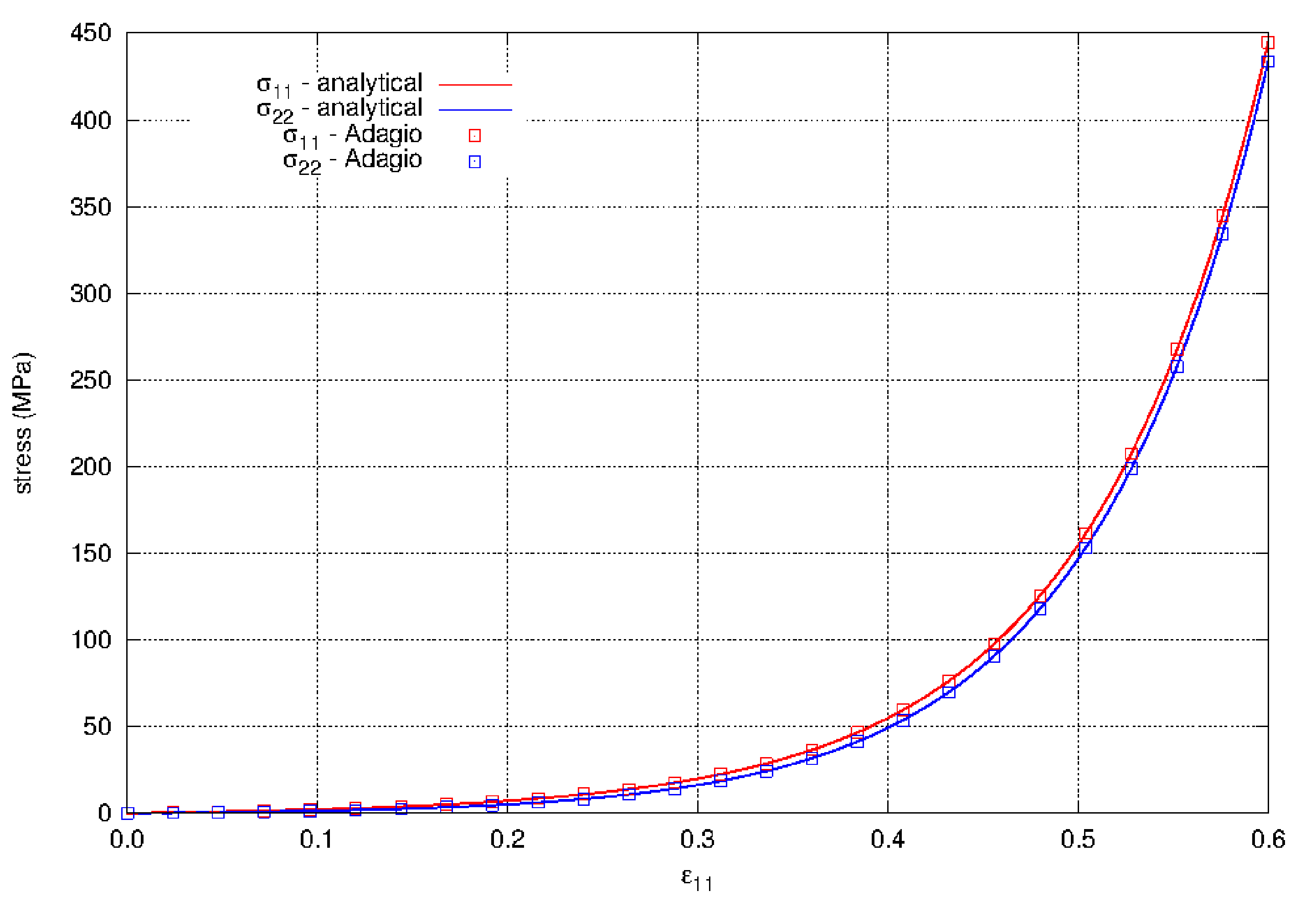
Fig. 4.105 The axial and lateral stresses for uniaxial strain in tension using the hyperfoam model. The results show agreement with the analytical results. The material properties for the model are given in Table 4.33

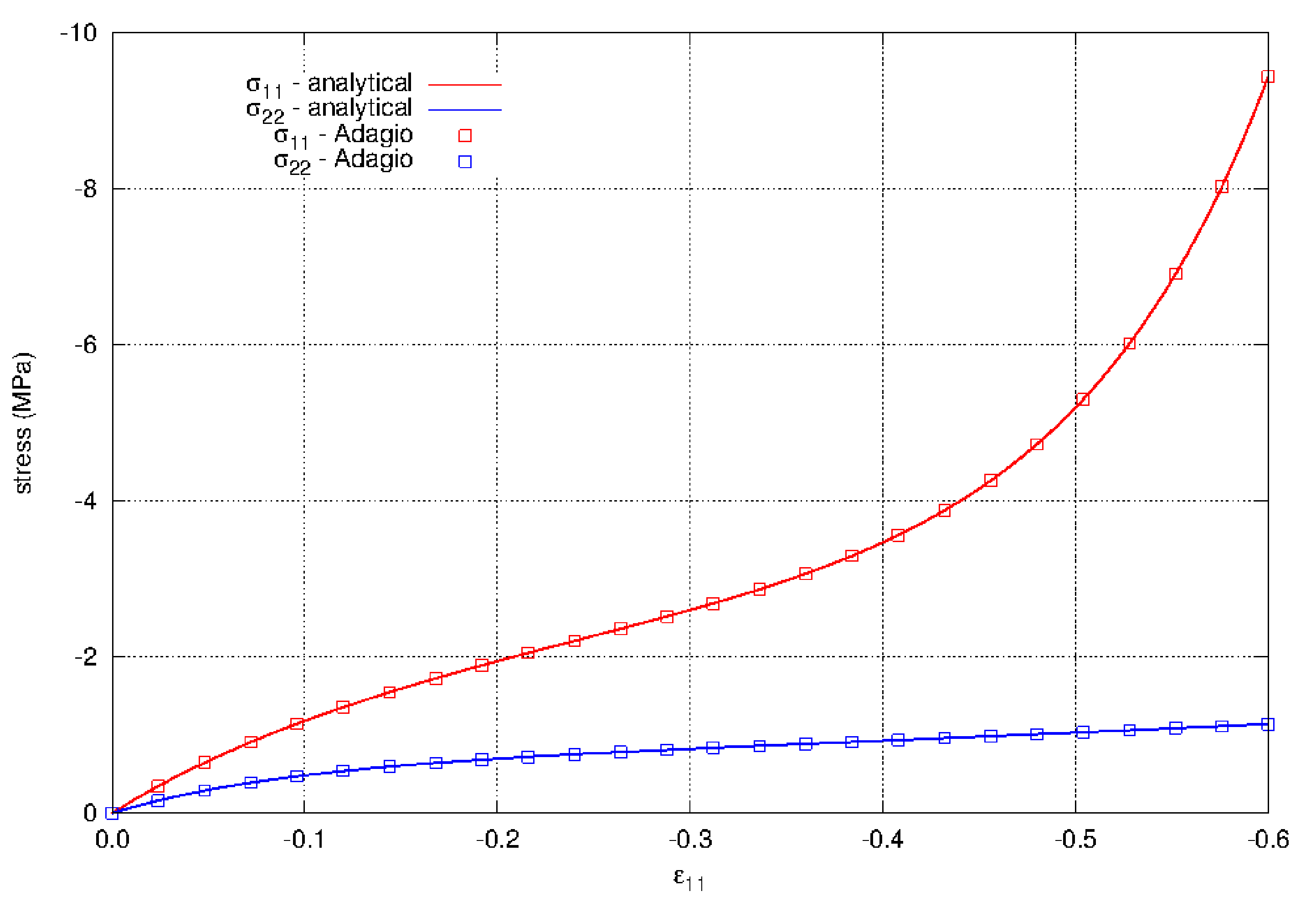
Fig. 4.106 The axial and lateral stresses for uniaxial strain in compression using the hyperfoam model. The results show agreement with the analytical results. The material properties for the model are given in Table 4.33.

Fig. 4.107 The axial and lateral stresses for uniaxial strain in both tension and compression using the hyperfoam model. The results show agreement with the analytical results and that the response of the material is very different in tension and compression. The material properties for the model are given in Table 4.33.

4.22.3.2. Biaxial Strain

Another simple verification problem for the hyperfoam model is biaxial strain.

In biaxial strain, the stretch ratios are prescribed in two orthogonal directions. For this \(\lambda_{1} = \exp(\varepsilon_{1})\) and \(\lambda_{2} = \exp(\varepsilon_{2})\), where \(\varepsilon_{i}\) are the applied strains in the \(x_{1}\) and \(x_{2}\) directions. In the third direction orthogonal to the first two, the stretch ratio is one. The determinant of the deformation gradient is \(J=\lambda_{1}\lambda_{2}\).

\[\begin{split}\sigma_{11} = \frac{1}{\lambda_{1}\lambda_{2}}\sum_{i=1}^{N}\frac{2\mu_{i}}{\alpha_{i}} \left[ \lambda_{1}^{\alpha_{i}}-\left(\lambda_{1}\lambda_{2}\right)^{-\alpha_{i}\beta_{i}} \right] \;\;\; ; \;\;\; \sigma_{22} = \frac{1}{\lambda_{1}\lambda_{2}}\sum_{i=1}^{N}\frac{2\mu_{i}}{\alpha_{i}} \left[ \lambda_{2}^{\alpha_{i}}-\left(\lambda_{1}\lambda_{2}\right)^{-\alpha_{i}\beta_{i}} \right] \nonumber \\ \\ \sigma_{33} = \frac{1}{\lambda_{1}\lambda_{2}} \sum_{i=1}^{N}\frac{2\mu_{i}}{\alpha_{i}} \left[ 1 - \left(\lambda_{1}\lambda_{2}\right)^{-\alpha_{i}\beta_{i}} \right] \nonumber\end{split}\]

The results of the analysis in tension are shown in Fig. 4.108 to Fig. 4.110.

For the results in Fig. 4.108, a single element is strained with \(\varepsilon_{1} = 0.4\) and \(\varepsilon_{2} = 0.2\) which, in biaxial strain in tension, is very large for this model. At some point the normal stresses begin to increase rapidly. Since the normal stresses are very large, the hydrostatic pressure is also very large. For this extreme loading the model in Adagio shows agreement with the analytical solution.

The model is also loaded in biaxial compression. These results are shown in Fig. 4.109. The model again shows agreement with the analytical solution. The behavior in compression is very different than tension. The maximum stress is orders of magnitude less at a strain of \(\varepsilon_{1} = -0.4\) and \(\varepsilon_{2} = -0.3\), where the maximum normal stress is just over 4.5 MPa, compared to \(\varepsilon_{1} = 0.4\) and \(\varepsilon_{2} = 0.3\) in tension where the normal stresses from the model are nearly 1.3 GPa. The lateral stress \(\sigma_{zz}\) reaches a plateau while the other two stress increase with increased straining The stresses in compression also have a different nonlinear form than the stresses in tension.

Finally, both the tension and compression responses are shown in Fig. 4.110. Here the continuity of the behavior at \(\varepsilon = 0\) can be seen along with the very different responses in tension and compression.

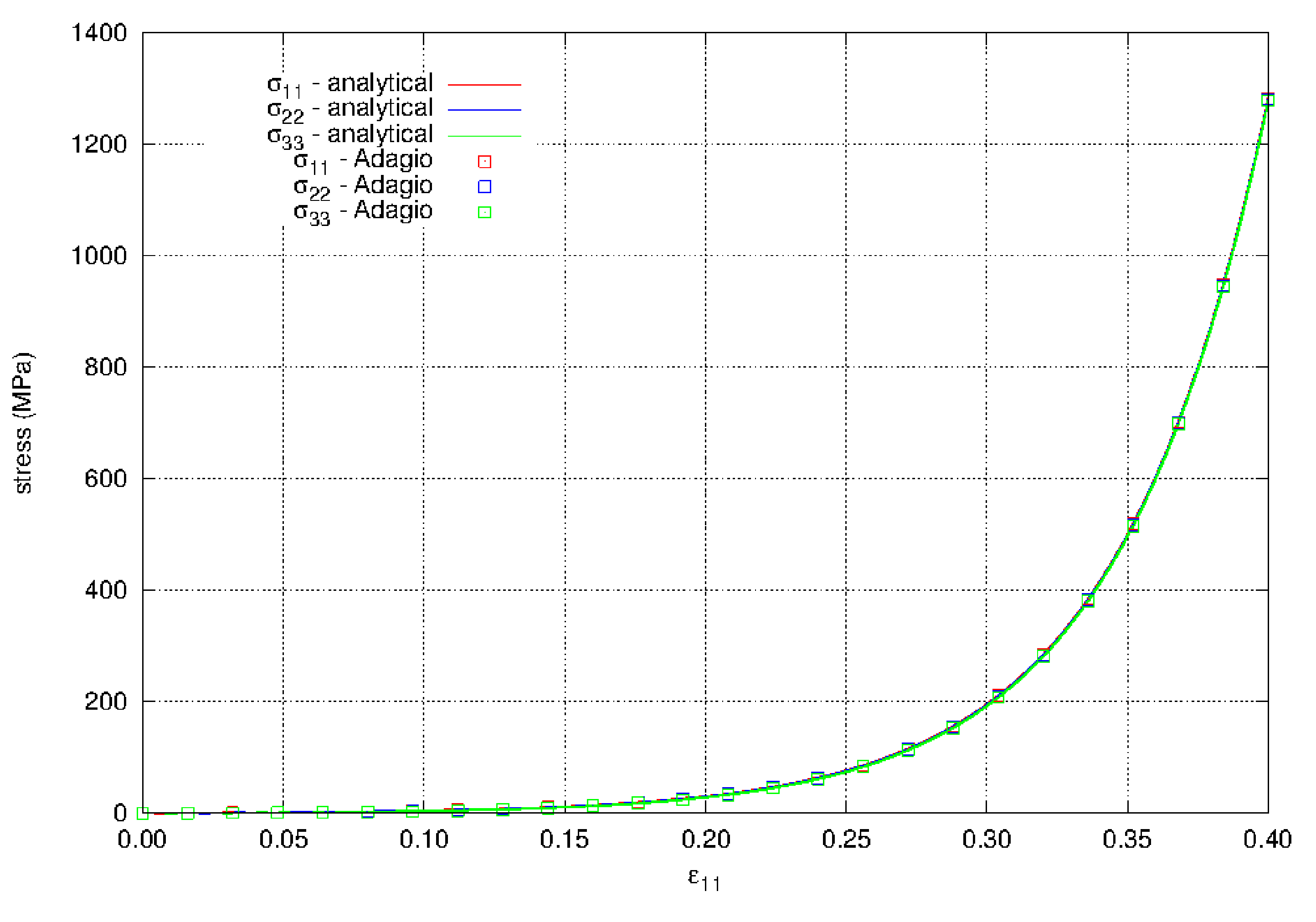
Fig. 4.108 The normal stresses for biaxial strain in tension using the hyperfoam model. The results show agreement with the analytical results. The material properties for the model are given in Table 4.33.

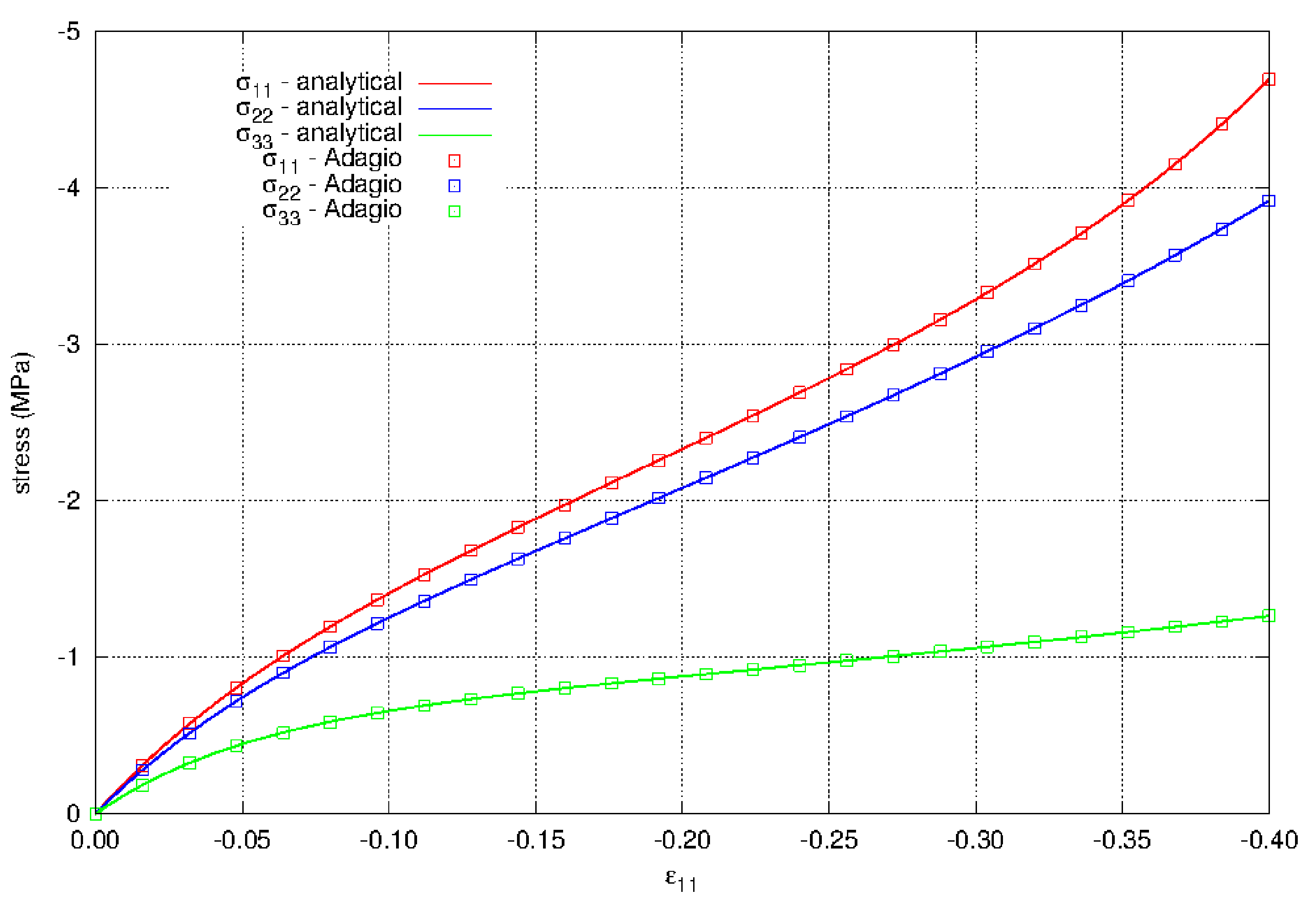
Fig. 4.109 The normal stresses for biaxial strain in compression using the hyperfoam model. The results show agreement with the analytical results. The material properties for the model are given in Table 4.33.

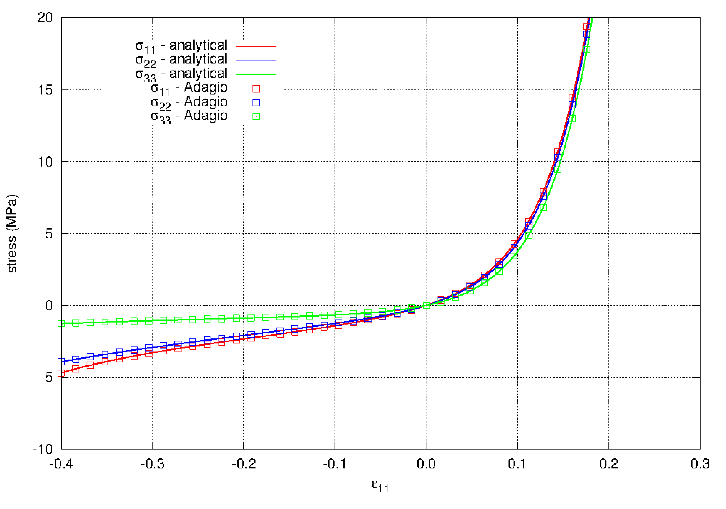
Fig. 4.110 The normal stresses for biaxial strain in both tension and compression using the hyperfoam model. The results show agreement with the analytical results and that the response of the material is very different in tension and compression. The material properties for the model are given in Table 4.33.

4.22.3.3. Pure Shear

The hyperfoam model is is also tested in pure shear in strain. Note that this is different from pure shear in stress.

In pure shear, the principal stretch ratios are \(\lambda_{1} = \lambda\), \(\lambda_{2} = 1\), and \(\lambda_{3} = \lambda^{-1}\). The determinant of the deformation gradient is \(J = 1\), which means the Kirchhoff and Cauchy stress measures are the same.

The principal stresses are

\[\sigma_{1} = \sum_{i=1}^{N}\frac{2\mu_{i}}{\alpha_{i}} \left(\lambda^{\alpha_{i}} - 1 \right) \;\;\; ; \;\;\; \sigma_{2} = 0 \;\;\; ; \;\;\; \sigma_{3} = \sum_{i=1}^{N}\frac{2\mu_{i}}{\alpha_{i}} \left( \lambda^{-\alpha_{i}} - 1 \right)\]

The principal axes of deformation are aligned at \(45^{\circ}\) to the coordinate axes. In the global coordinate system the non-zero stress components are

\[\begin{split}\sigma_{11} = \sigma_{22} = \sum_{i=1}^{N}\frac{2\mu_{i}}{\alpha_{i}} \left(\lambda^{\alpha_{i}} + \lambda^{-\alpha_{i}} - 2 \right) \nonumber \\ \\ \sigma_{12} = \sum_{i=1}^{N}\frac{2\mu_{i}}{\alpha_{i}} \left( \lambda^{\alpha_{i}} - \lambda^{-\alpha_{i}} \right) \nonumber\end{split}\]

The results of the analysis in pure shear are shown in Fig. 4.111. A single element is strained to a shear strain of \(\varepsilon = 0.4\). The model in Adagio shows agreement with the analytical solution presented above. It is interesting to note that pure shear strain produces not only normal stresses with the hyperfoam model, but a non-zero pressure. The deviatoric/volumetric split so often used with our constitutive model does not occur with the hyperfoam model.

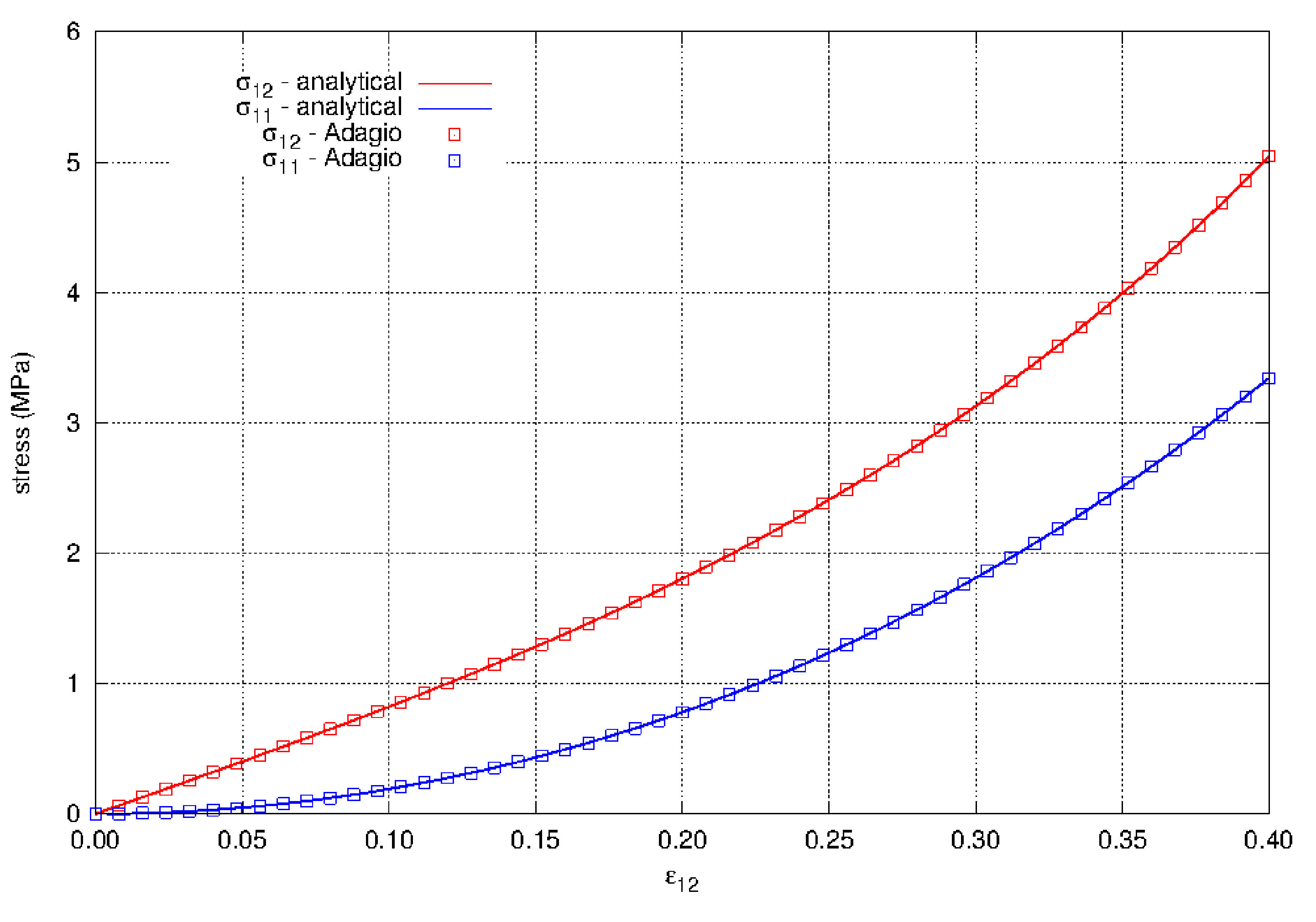
Fig. 4.111 The shear and normal stresses for the hyperfoam model in pure shear. The material properties for the model are given in Table 4.33.

4.22.3.4. Simple Shear

The hyperfoam model is is also tested in simple shear. Note that this is a different deformation path than pure shear. In simple shear the deformation gradient is

\[\begin{split}\left[ F_{ij} \right] = \begin{bmatrix} 1 & \gamma & 0 \\ 0 & 1 & 0 \\ 0 & 0 & 1 \end{bmatrix}\end{split}\]

The principal stretch ratios are \(\lambda_{1} = \lambda\), \(\lambda_{2} = 1\), and \(\lambda_{3} = \lambda^{-1}\). The determinant of the deformation gradient is \(J = 1\), which means the Kirchhoff and Cauchy stress measures are the same. This gives the {em same} principal stresses as in pure shear when written in terms of the principal stretch ratio, \(\lambda\). The principal stresses are

\[\sigma_{1} = \sum_{i=1}^{N}\frac{2\mu_{i}}{\alpha_{i}} \left(\lambda^{\alpha_{i}} - 1 \right) \;\;\; ; \;\;\; \sigma_{2} = 0 \;\;\; ; \;\;\; \sigma_{3} = \sum_{i=1}^{N}\frac{2\mu_{i}}{\alpha_{i}} \left( \lambda^{-\alpha_{i}} - 1 \right)\]

The principal stretch ratio is

\[\lambda = \frac{1 + \sin\theta}{\cos\theta} \;\;\; ; \;\;\; \theta = \tan^{-1}\left( \frac{\gamma}{2} \right)\]

The principal axes of deformation in the current configuration, i.e. the eigenvectors of the left stretch, are given by

\[\hat{e}^{1}_i = \cos\phi \, {e}^{1}_i + \sin\phi \, {e}^{2}_i \;\;\; ; \;\;\; \hat{e}^{2}_i = {e}^{3}_i \;\;\; ; \;\;\; \hat{e}^{3}_i = -\sin\phi \, {e}^{1}_i + \cos\phi \, {e}^{2}_i\]

where \(\phi = \pi/4 - \theta/2\).

The results of the analysis in simple shear are shown in Fig. 4.112. A single element is strained to a shear parameter of \(\gamma = 0.4\). The model in Adagio shows agreement with the analytical solution presented above. It is interesting to note that simple shear with the hyperfoam model produces different normal stresses than simple shear, i.e. the two non-zero normal stresses are not equal. The difference arises from the fact that the principal axes of deformation in pure shear are fixed, while in simple shear the principal axes rotate. There is still a non-zero pressure which again shows that the deviatoric/volumetric split does not occur with the hyperfoam model.

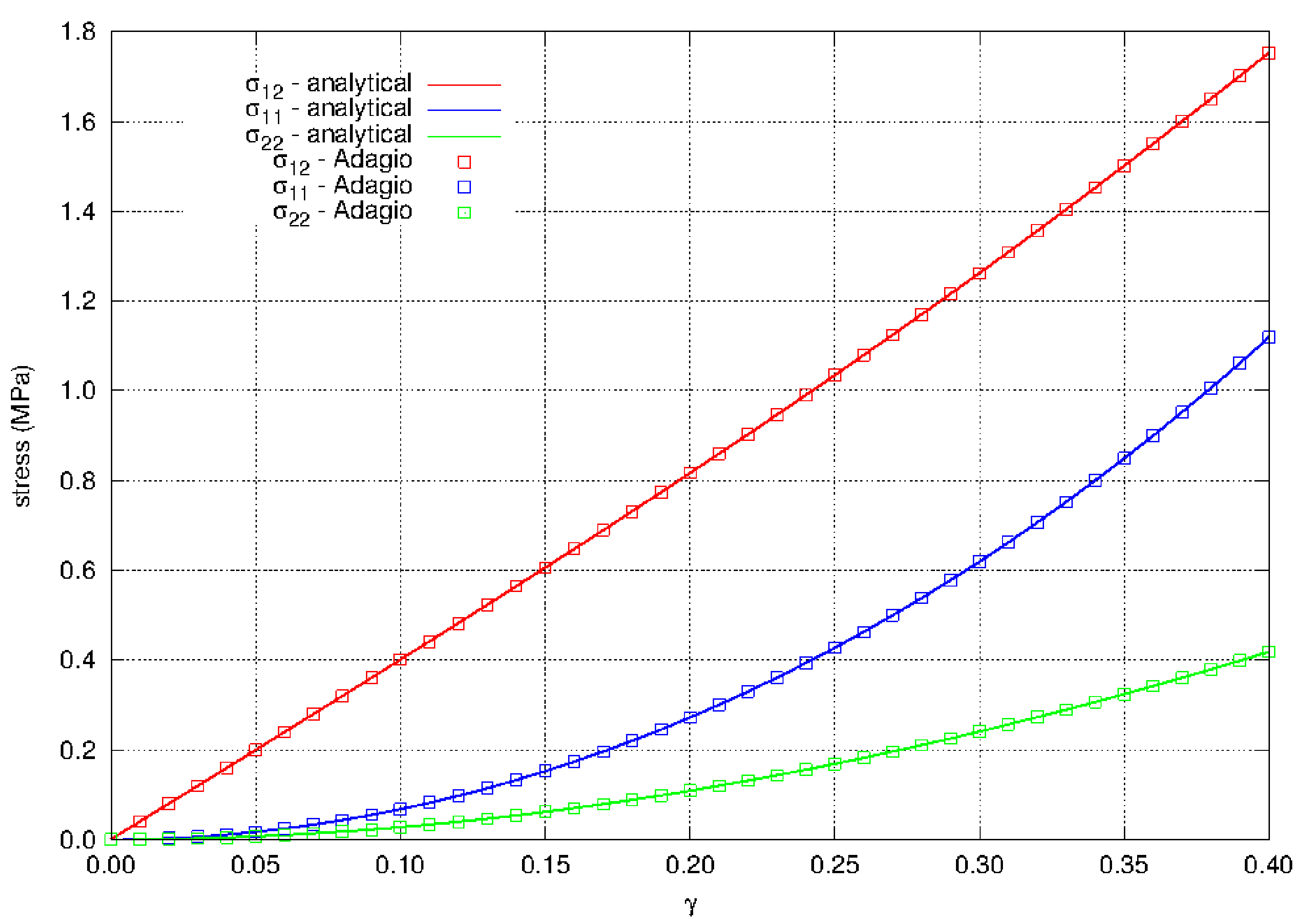
Fig. 4.112 The shear and normal stresses for the hyperfoam model in simple shear. The material properties for the model are given in Table 4.33.

4.22.4. User Guide

BEGIN PARAMETERS FOR MODEL HYPERFOAM
  #
  # Elastic constants
  #
  YOUNGS MODULUS = <real>
  POISSONS RATIO = <real>
  SHEAR MODULUS  = <real>
  BULK MODULUS   = <real>
  LAMBDA         = <real>
  TWO MU         = <real>
  #
  # Strain energy density
  #
  N = <integer>
  SHEAR    = <real_list>
  ALPHA    = <real_list>
  POISSON  = <real_list>
END [PARAMETERS FOR HYPERFOAM]

• The number of terms in the expansion of the strain energy is defined with the N command line.

• The shear terms in the expansion of the strain energy, \(\mu_{i}\), are defined with the SHEAR command line.

• The alpha terms in the expansion of the strain energy, \(\alpha_{i}\), are defined with the ALPHA command line.

• The Poisson ratio terms in the expansion of the strain energy, \(\nu_{i}\), are defined with the POISSON command line.

There are no output variables available for this model.

---

[1]

B. Störakers. On material representation and constitutive branching in finite compressible elasticity. Journal of the Mechanics and Physics of Solids, 34:125–145, 1986.

[2]

R. W. Ogden. Non-Linear Elastic Deformaitons. Dover, New York, 1984.

[3]

P. J. Blatz and W. L. Ko. Application of finite elasticity theory to the deformation of rubbery materials. Transactions of the Society of Rheology, 6:223–251, 1962.

[4]

G. Bolzon and R. Vitaliani. The blatz-ko model and homogenization. Archive of Applied Mechanics, 63:228–241, 1993.