4.28. Viscoplastic Foam Model

4.28.1. Theory

The viscoplastic foam model is used to model the rate (and temperature) dependent crushing of foams [[1]]. It is based on an additive split of the rate of deformation into an elastic and plastic portion

\[D_{ij} = D^{\text{e}}_{ij} + D^{\text{p}}_{ij}.\]

The stress in the material is due strictly to the elastic portion of the rate of deformation so that

\[\stackrel{\circ}{\sigma}_{ij} = \mathbb{C}_{ijkl}D^{\text{e}}_{kl},\]

where \(\mathbb{C}_{ijkl}\) are the components of the fourth-order, isotropic elasticity tensor. The stress rate is arbitrary, as long as it is objective. Two objective stress rates are commonly used: the Jaumann rate and the Green-McInnis rate. For problems with fixed principal axes of deformation, these two rates give the same answers. For problems where the principal axes of deformation rotate during deformation, the two rates can give different answers.

To describe the rate-dependent response, an over-stress-type yield function is used. Specifically, the rate-independent foam plasticity yield function

(4.133)\[f=\frac{\bar{\sigma}^2}{a^2}+\frac{p^2}{b^2}-1\]

where \(\sigma^*\) is the effective stress given by

(4.134)\[\sigma^*=\sqrt{\bar{\sigma}^2+\frac{a^2}{b^2}p^2}.\]

In (4.134), \(\bar{\sigma}\) is the von Mises effective stress (\(\bar{\sigma}=\sqrt{\frac{3}{2}s_{ij}s_{ij}}\)) and \(p\) is the pressure resulting from a stress decomposition of the form,

\[s_{ij}=\sigma_{ij}-p\delta_{ij}.\]

Furthermore, \(a\) and \(b\) are state variables that are functions of the absolute temperature, \(\theta\), and maximum solid volume fraction, \(\phi\), and are defined as

(4.135)\[a\left(\theta,\phi\right) = \left(A_{0}\left(\theta\right) + A_{1}\left(\theta\right)\phi^{A_{2}}\right)f_a\left(\phi\right),\]

(4.136)\[b\left(\theta,\phi\right) = \left(B_{0}\left(\theta\right) + B_{1}\left(\theta\right)\phi^{B_{2}}\right)f_b\left(\phi\right).\]

In (4.135) and (4.136), the functional forms are chosen to provide flexibility in terms of representation. To this end, \(f_a\) and \(f_b\) default to constant values of one and the expression reduce to legacy analytical functions. This both provides for backward compatibility with previous user input decks while allowing for user defined definitions. Further, if \(A_1\left(\theta\right)=0\), \(a\left(\theta,\phi\right)=A_0\left(\theta\right)f_a\left(\phi\right)\); a multiplicative decomposition of dependencies.

The temperature dependent material properties in the preceding relations are all defined as, \(A_{0}\left(\theta\right)=A_0h_{A_0}\left(\theta\right)\) where \(A_0\) is the reference material parameter and \(h_{A_0}\left(\theta\right)\) is the relative value as a function of temperature. In addition to the \(a\) and \(b\) state variables, the Young’s modulus and Poisson’s ratio are also functions of the absolute temperature. The latter may be written as \(\nu\left(\theta\right)=\nu h_{\nu}\left(\theta\right)\) while the former is also dependent on the maximum volume fraction of solid material and is given as \(E\left(\theta,\phi\right)=Eh_E\left(\theta\right)f_E\left(\phi\right)\).

The maximum volume fraction of solid material, \(\phi\), is given by

\[\phi=\max_{t>0}\tilde{\phi}\left(t\right)\]

where \(\tilde{\phi}\left(t\right)\) is the current volume fraction of solid material and is defined as,

\[\tilde{\phi}\left(t\right) = \frac{\phi_{0}}{\exp\left(\varepsilon^{\text{p}}_v\right)}\]

with \(\phi_0\) being the initial solid volume fraction and \(\varepsilon^{\text{p}}_v\) is

\[\varepsilon^{\text{p}}_v = \int_{0}^{t} D_{kk}^{\text{p}} dt.\]

During inelastic deformation (\(f>0\)), the corresponding rate of plastic deformation is given in a Perzyna-type form as,

\[\begin{split}D_{ij}^{\text{p}} = \left\{ \begin{array}{ccc} \displaystyle{\exp\left(h\left(\theta\right)\right)\left( \frac{\sigma^{*}}{a} - 1 \right)^{n\left(\theta\right)}g_{ij}} & \mbox{if} & f > 0 \\ & & \\ 0 & \mbox{if} & f \leq 0 \\ \end{array} \right.\end{split}\]

where \(h\left(\theta\right)\) and \(n\left(\theta\right)\) are the flow rate and power exponent respectively. The inelastic flow direction, \(g_{ij}\), is given as a linear combination of the associated (with respect to (4.133)), \(g^{\text{a}}_{ij}\), and radial, \(g^{\text{r}}_{ij}\),

(4.137)\[g_{ij}=\frac{\left(1-\beta\right)g_{ij}^{\text{a}}+\beta g_{ij}^{\text{r}}}{|\left(1-\beta\right)g_{kl}^{\text{a}}+\beta g_{kl}^{\text{r}}|}\]

The directions \(g^{\text{a}}_{ij}\) and \(g^{\text{r}}_{ij}\) are given by

\[\begin{split}g^{\text{a}}_{ij} & =\frac{\frac{\partial f}{\partial \sigma_{ij}}}{|\frac{\partial f}{\partial\sigma_{kl}}|} = \frac{\frac{3}{a^2}s_{ij}-\frac{2}{3b^2}p\delta_{ij}}{|\frac{3}{a^2}s_{ij}-\frac{2}{3b^2}p\delta_{ij}|},\\ g^{\text{r}}_{ij} & = \frac{\sigma_{ij}}{|\sigma_{kl}|}=\frac{\sigma_{ij}}{\sqrt{\sigma_{kl}\sigma_{kl}}},\end{split}\]

in Equations (4.129) and (4.130),

respectively. In this model, the flow rule weight, \(\beta\), may be specified as either a constant value or as a function of the maximum solid volume fraction (\(\beta=\beta_0f_{\beta}\left(\phi\right)\)).

4.28.2. Implementation

As the viscoplastic foam model is a time-dependent, hypoelastic model it is integrated using an explicit, forward Euler scheme. Given this approach, a critical time step for stability is computed based on the shear strength, current modulus, and deviatoric deformation rate. If the input time step is acceptable, the new material state at time \(t=t_{n+1}\) is computed. On the other hand, if the time step is too large a series of sub-increments are used. In this case, the total time step \(\Delta t\) is subdivided into \(N\) sub-increments. Each such sub-interval (denoted by \(k\)) has a time increment \(\delta t^k\) such that \(\Delta t = \sum_{k=1}^{N}\delta t^k\) and the forward Euler time stepping scheme is performed over each sub-interval until the desired material state at time \(t_{n+1}\) is determined. For the case of temperature dependent variables (e.g. the Poisson’s ratio \(\nu\)), the value at the start of the sub-increment is determined by linearly interpolating over the total time step,

\[\nu^k=\nu_n+\frac{\Delta t^k}{\Delta t}\left(\nu_{n+1}-\nu_{n}\right),\]

where \(\Delta t^k\) is the current sub-increment time, \(\Delta t^k=\sum_{r=1}^k\delta t^r\). For simplicity, in the remainder of this section it is assumed that the input time step is acceptable and only a single increment is needed. If additional sub-increments are needed, the below steps would be repeated \(N\) times with time intervals of \(\delta t^k\).

Noting the forward Euler approach adopted in this formulation, the first step is to determine the temperature (and solid volume fraction) dependent model parameters (\(E,~\nu,~A_0,~A_1,~B_0,~B_1,~h\) and \(n\)). With the parameters established, state variables \(a\) and \(b\) are easily determined through (4.135) and (4.136), respectively, enabling the calculation of the effective stress via (4.134). The effective inelastic (plastic) strain rate, \(\dot{\bar{\varepsilon}}^p\), is then given as,

\[\dot{\bar{\varepsilon}}^p=\exp\left(h\left(\theta_n\right)\right)\left<\frac{\sigma^*_n}{a_n}-1\right>^{n\left(\theta_n\right)},\]

with \(\left< \right>\) being the Macaulay brackets such that,

\[\begin{split}\left<x\right>=\left\{\begin{array}{cc} x & x \geq 0 \\ 0 & x < 0\end{array}\right..\end{split}\]

Knowing the magnitude of the rate of inelastic deformation, the change in deviatoric and hydrostatic stresses is simply,

\[\begin{split}\dot{s}_{ij}=2\mu\left(\theta_n,\phi_n\right)\left(\hat{d}_{ij}-\hat{d}^{\text{p}}_{ij}\right), \\ \dot{p}=K\left(\theta_n,\phi_n\right)\left(d_{kk}-d^{\text{p}}_{kk}\right),\end{split}\]

where \(d_{ij}\) is the total unrotated rate of deformation, \(\hat{x}_{ij}\) denotes the deviatoric portion of tensor \(x_{ij}\), and \(d^{\text{p}}_{ij}\) is the plastic rate of deformation given by,

(4.138)\[d^{\text{p}}_{ij}=\dot{\bar{\varepsilon}}^pg^n_{ij}.\]

In (4.138), \(g_{ij}\) is the inelastic flow direction and can be calculated via (4.137).

An additional comment is needed with respect to accounting for temperature and solid volume fraction dependence in the shear and bulk moduli. This careful consideration is necessary due to the fact that the temperature dependence is only given with respect to the elastic moduli and Poisson’s ratio. As such, the shear and bulk moduli inherit the associated dependencies and are calculated for isotropic elastic relations. For the bulk moduli, this leads to an expression of the form,

\[K\left(\theta,\phi\right)=\frac{Eh_E\left(\theta\right)f_E\left(\phi\right)}{3\left(1-2\nu h_{\nu}\left(\theta\right)\right)}.\]

The updated stress state is then easily computed by explicitly integrating the established expressions. Specifically,

\[\begin{split}s^{n+1}_{ij}=\frac{\mu_{n+1}}{\mu_{n}}s_{ij}^n+\dot{s}_{ij}\Delta t, \\ p^{n+1}=\frac{K_{n+1}}{K_n}p^n+\dot{p}\Delta t, \\ T^{n+1}_{ij}=s^{n+1}_{ij}+p^{n+1}\delta_{ij},\end{split}\]

with \(\mu_n\) and \(K_n\) representing \(\mu\left(\theta_n,\phi_n\right)\) and \(K\left(\theta_n,\phi_n\right)\), respectively, and \(T_{ij}\) being the unrotated stress.

4.28.3. Verification

The viscoplastic foam model was verified in both uniaxial and hydrostatic compression. The material properties and model parameters for both of these investigations are given in Table 4.43. As both loadings are isothermal, temperature dependence is neglected in the relevant model parameters. Furthermore, analytical solutions could not be found directly, so semi-analytical solutions were found.

Table 4.43 The material properties for the viscoplastic foam model tested in uniaxial stress.

\(E\)	4,807 psi	\(A_{0}\)	63.03 psi
\(\nu\)	0.33	\(A_{1}\)	7000 psi
\(h\)	-8.12	\(A_{2}\)	3.7878
\(n\)	2	\(B_{0}\)	93 psi
\(\beta\)	0.9	\(B_{1}\)	1483.4 psi
\(\phi_{0}\)	0.1148	\(B_{2}\)	3.7878

4.28.3.1. Uniaxial Compression

To obtain a semi-analytical solution for the uniaxial compression test, the model was reduced to a one-dimensional form and then numerically integrated. The results obtained from the implemented model and the semi-analytical solution are shown below in Fig. 4.124.

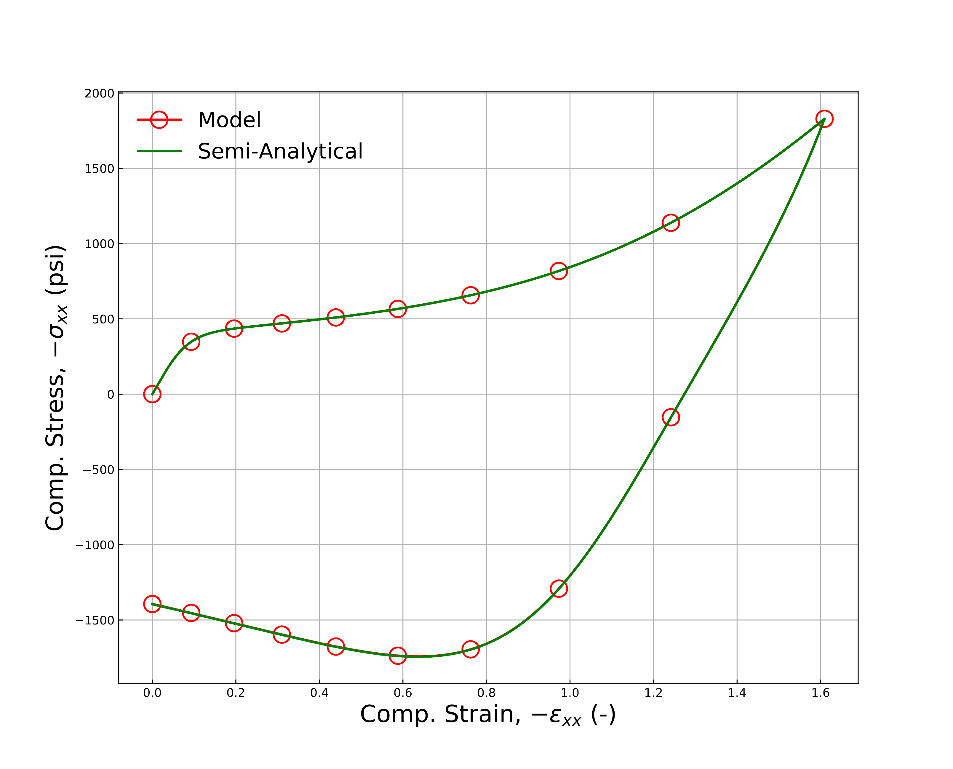
Fig. 4.124 Verification of the viscoplastic foam model in uniaxialcompression showing the axial stress as a function of thelogarithmic strain

4.28.3.2. Hydrostatic Compression

The response of the model through hydrostatic compression. To this end, a displacement of the form \(u_i=\lambda\left(t\right)\) is considered. The applied displacement scales linearly from \(\lambda=0\) at \(t=0.0\) to \(\lambda=-0.7\) at \(t=t_{\text{max}}\). Rate-dependent effects are considered through the use of two cases each with a different \(t_{\text{max}}\). Creatively denoted Fast and Slow, the two cases correspond to \(t_{\text{max}}=1\) s and \(t_{\text{max}}=100\) s, respectively. With such a displacement field, the engineering volume strain, \(\varepsilon_{\text{V}}\), is simply \(\varepsilon_{\text{V}}=\left(1+\lambda\right)^3-1\). Additionally, the stress state reduces trivially to \(\sigma_{ij}=-p\delta_{ij}\).

Given the rate-dependent overstress form of the constitutive model, an analytical solution is not readily available. Therefore, a semi-analytical analysis using a model reduction specialized for hydrostatic loadings is considered. Specifically, noting \(s_{ij}=0\), the overstress reduces to,

\[\sigma^*=\frac{a}{b}|p|.\]

Furthermore, the associated and radial flow direction vectors simplify to the same form and are given as,

\[g^{\text{a}}_{ij}=g^{\text{r}}_{ij}=-\frac{1}{\sqrt{3}}\text{sgn}\left(p\right)\delta_{ij},\]

where \(\text{sgn}\left(p\right)\) is the sign of \(p\). The semi-analytical (integrated in a forward Euler fashion) and numerical results are presented in Fig. 4.125.

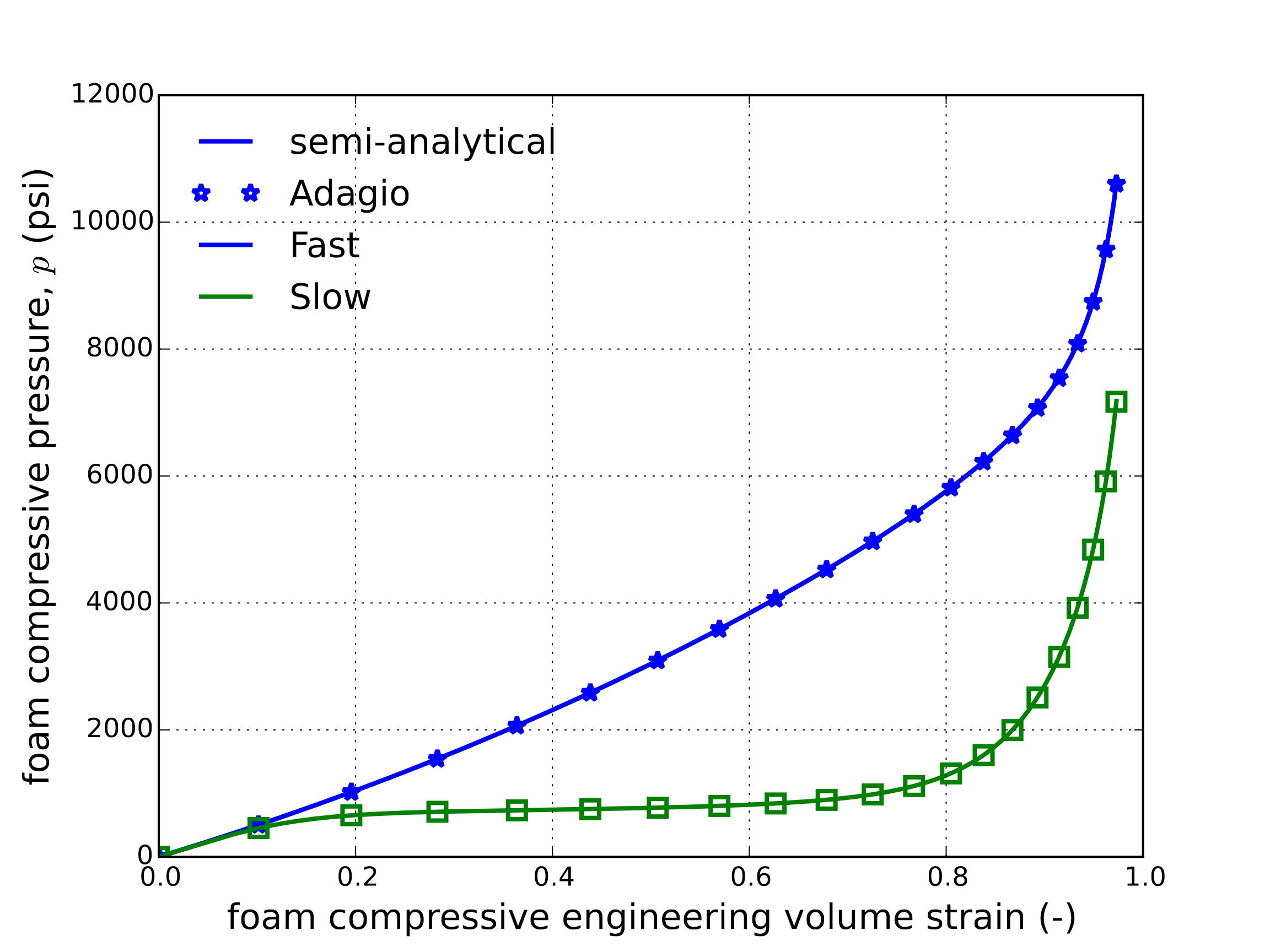
Fig. 4.125 Pressure-engineering volume strain results of viscoplastic foam model subjected to a hydrostatic loading at both fast and slow rates determined semi-analytically and numerically.

4.28.4. User Guide

BEGIN PARAMETERS FOR MODEL VISCOPLASTIC_FOAM
  #
  # Elastic constants
  #
  YOUNGS MODULUS = <real>
  POISSONS RATIO = <real>
  SHEAR MODULUS  = <real>
  BULK MODULUS   = <real>
  LAMBDA         = <real>
  TWO MU         = <real>

  FLOW RATE      = <real>
  POWER EXPONENT = <real>
  BETA           = <real> (1.0)
  PHI            = <real>

  SHEAR STRENGTH  = <real> (1.0)
  SHEAR HARDENING = <real> (0.0)
  SHEAR EXPONENT  = <real> (1.0)
  HYDRO STRENGTH  = <real> (1.0)
  HYDRO HARDENING = <real> (0.0)
  HYDRO EXPONENT  = <real> (1.0)

  YOUNGS FUNCTION    = <string>
  POISSONS FUNCTION  = <string>
  SS FUNCTION        = <string>
  SH FUNCTION        = <string>
  HS FUNCTION        = <string>
  HH FUNCTION        = <string>
  RATE FUNCTION      = <string>
  EXPONENT FUNCTION  = <string>
  STIFFNESS FUNCTION = <string>

  SHEAR HARDENING FUNCTION = <string>
  HYDRO HARDENING FUNCTION = <string>
  BETA FUNCTION            = <string>
END [PARAMETERS FOR MODEL VISCOPLASTIC_FOAM]

In the above command blocks:

• Since the model requires functions to describe the temperature dependence of the elastic modulus and Poisson’s ratio, it is recommended that one inputs these properties at some reference temperature. However, any two of the elastic constants can be used for input.

• The reference value for the flow rate, \(h\), is defined with the FLOW RATE command line.

• The reference value of the over-stress exponent, \(n\), is defined with the POWER EXPONENT command line.

• The user-defined scalar scaling between associated and radial flow, \(\beta\), is defined with the BETA command line.

• The initial volume fraction of solid material, \(\phi_0\), is defined with the PHI command line.

• The reference value for the shear strength, \(A_{0}\), is defined with the SHEAR STRENGTH command line.

• The reference value for the shear hardening modulus, \(A_1\), is defined with the SHEAR HARDENING command line.

• The shear hardening exponent, \(A_{2}\), is defined with the SHEAR EXPONENT command line.

• The reference value for the hydrostatic strength, \(B_{0}\), is defined with the HYDRO STRENGTH command line.

• The reference value for the hydrostatic hardening modulus, \(B_{1}\), is defined with the HYDRO HARDENING command line.

• The hydrostatic hardening exponent, \(B_{2}\), is defined with the HYDRO EXPONENT command line.

• The user-defined and normalized function that gives the elastic modulus as a function of temperature, \(h_{E}(\theta)\), is defined with the YOUNGS FUNCTION command line.

• The user-defined and normalized function that gives the Poisson’s ratio as a function of temperature, \(h_{\nu}(\theta)\), is defined with the POISSONS FUNCTION command line.

• The user-defined and normalized function that gives the shear strength as a function of temperature, \(h_{A_0}(\theta)\), is defined with the SS FUNCTION command line.

• The user-defined and normalized function that gives the shear hardening modulus as a function of temperature, \(h_{A_1}(\theta)\), is defined with the SH FUNCTION command line.

• The user-defined and normalized function that gives the hydrostatic strength as a function of temperature, \(h_{B_0}(\theta)\), is defined with the HS FUNCTION command line.

• The user-defined and normalized function that gives the hydrostatic hardening modulus as a function of temperature, \(h_{B_1}(\theta)\), is defined with the HH FUNCTION command line.

• The user-defined and normalized function that gives the flow rate as a function of temperature, \(h_{h}(\theta)\), is defined with the RATE FUNCTION command line.

• The user-defined and normalized function that gives the over-stress exponent as a function of temperature, \(h_{n}(\theta)\), is defined with the EXPONENT FUNCTION command line.

• The user-defined and normalized function that gives the elastic modulus as a function of maximum solid volume fraction, \(f_{E}(\phi)\), is defined with the STIFFNESS FUNCTION command line.

• The optional user-defined function that gives the shear strength as a function of the maximum solid volume fraction, \(a\left(\phi\right)\), is defined with the SHEAR HARDENING FUNCTION command line. Note, if this function is defined the SHEAR STRENGTH, SHEAR HARDENING, and SHEAR EXPONENT values should not be specified.

• The optional user-defended function that gives the hydrostatic strength as a function of the maximum solid volume fraction, \(b\left(\phi\right)\), is defined with the HYDRO HARDENING FUNCTION command line. Note, if this function is defined the HYDRO STRENGTH, HYDRO HARDENING, and HYDRO EXPONENT values should not be specified.

• The optional user-defined function that gives the scaling between associated and radial flow as a function of maximum solid volume fraction, \(\beta\left(\phi\right)\), is defined with the BETA FUNCTION command line. Note, if this function is defined the BETA value should not be specified.

Output variables available for this model are listed in Table 4.44.

Table 4.44 State Variables for VISCOPLASTIC FOAM Model

Name	Description
ITER	number of sub-increments
EPVOL	inelastic volumetric strain, \(\varepsilon^{\text{p}}_v\)
EDOT	effective inelastic strain rate, \(\dot{\bar{\varepsilon}}^{p}\)
PHI	maximum volume fraction of solid material, \(\phi\)
FA	shear strength, \(a\)
FB	hydrostatic strength, \(b\)
STIF	elastic stiffness as a function of \(\phi\)

---

[1]

M. K. Neilsen, W. Y. Lu, B. Olsson, and T. Hinnerichs. A viscoplastic constitutive model for polyurethane foams. In Proceedings ASME 2006 International Mechanical Engineering Congress and Exposition. Chicago, IL, 2006. ASME.