
6. Superelements#
Superelements can greatly reduce the computational cost of large model. But they are hard to use. Recall from Section 5 that in Sierra/SD we have no automatic superelement capability. Superelements are usually used as follows.
A full sized, complete model is generated.
Portions of the model are extracted, and a reduced CBR model is created from that extracted model.
The full model is modified by removing the extracted portions and replacing each with a superelement.
The modified model is analyzed.
The modified model is post processed.
This section describes each step for a realistic example.
6.1. Superelement Example#
The full model is shown in Figure 6.1. The model consists of the following.
A lower leg portion consisting of two solid blocks and several beam blocks for applying loads and tying the model together. This will become superelement 1.
A central joint section representing the bolted joint. The joint is nonlinear, and is the primary interest in the study. It is a single, zero length beam that is attached to the upper and lower leg sections. This will not become a superelement.
An upper leg section that is similar to the lower leg. This will become superelement 2.
Id |
# elements |
type |
SE |
color |
Description |
|---|---|---|---|---|---|
81 |
188 |
bar |
1 |
blue |
lower load spreading network |
11 |
11072 |
Hex20 |
1 |
red |
lower support block |
12 |
2158 |
Hex20 |
1 |
pink |
lower joint support |
51 |
54 |
bar |
1 |
cyan |
joint connection network |
53 |
1 |
bar |
none |
red |
joint |
52 |
124 |
bar |
none |
blue |
joint connection network |
21 |
15024 |
Hex20 |
2 |
yellow |
upper joint support |
22 |
2106 |
Hex20 |
2 |
green |
upper support block |
82 |
184 |
bar |
none |
purple |
load spreading network |
Note: blocks 61, 62, 63, 71, 72, 72 are not shown and connect the Hex blocks
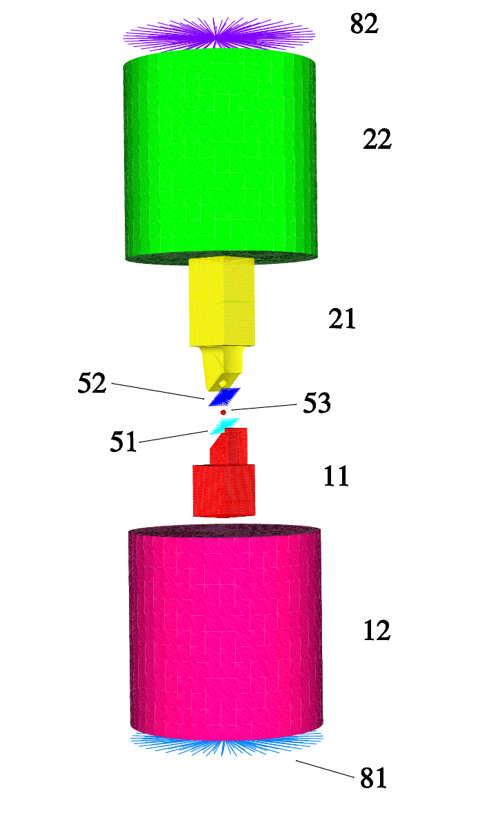 Exploded view of model
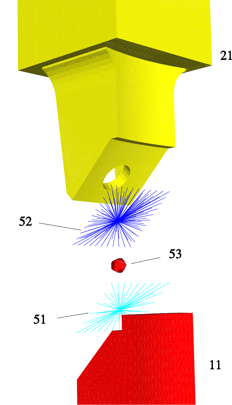 Zoom view of joint
Figure 6.1 Superelement model: (a) exploded view of model and (b) zoom view of joint.#
The two superelements are attached in very different ways to illustrate the issues introduced by the connections. The lower model has only two interface nodes, at the centers of the networks 81 and 51. This makes a small structure that is easy to interface. However, because the interface nodes may not be part of an MPC, it also requires that these two networks be beams rather than the rigid Rbars that the analyst would prefer.
In contrast, the upper superelement uses Rbars, but they must be put in the residual structure. Thus, blocks 52 and 82 are not part of the superelement. The consequence is that there are many interface degrees of freedom which greatly complicates interfacing to the superelement, and significantly increases the computational cost of the model reduction.
The joint model (block 53) consists of a single Joint2G element.
Topographically this is a 2 noded bar element which will be used to
control the translations and rotations of the two points. Block 53 is
connected to the centers of the two network blocks (51 and 52) which
connect to the lower and upper joint supports respectively.
6.2. Submodel Model Extraction and Reduction#
The two main ways of extracting a submodel from the original full model are to either 1) build up the submodel from scratch, or 2) pull the model out of the original model. When the model interface is complex, I would strongly recommend the second method. This is because it is complicated to assign the interface nodes to the revised model when the superelement is reinserted (see section 6.3). If the node number does not change between these two models, then this book keeping is minimized.
Extracting portions of a system model for CBR reduction may be done using the Grepos utility which preserves the node ordering.
$ grepos input.exo output.exo
GREPOS> delete block all
GREPOS> undelete block 1
GREPOS> exit
6.2.1. SE1: The lower structure with a small interface#
For this model I went into Patran and removed all the elements except those in blocks 11, 12, 51, 61, 62, 63 and 81. [1] In hindsight removing blocks is easier with Grepos than Patran. To define the interface, I defined nodeset 1111 at the center of the networks in blocks 51 and 81. I removed all other nodeset and sidesets, and all empty block definitions. Nodeset 100 was created at random points for an OTM, and the elements were renumbered. No nodes were removed.
A “check” of this model in explore indicates that there are 77726
nodes that are not connected to any element. This is as expected, and
there are no other errors reported.
The model is split into 10 regions using stk_balance, and model
reduction is performed on our Linux cluster (liberty). Run times are
shown below. Each processor required about 450MB of memory.
step |
elapsed time |
comment |
|---|---|---|
matrix assembly |
00:12 |
|
CBR restructure |
03:58 |
|
fixed interface modes |
20:44 |
computed 50 eigenvalues |
constraint modes |
25:43 |
computed 12 constraint modes |
model reduction |
25:43 |
|
total (10 processors) |
25:43 |
model size: 186 kB |
6.2.2. SE2: The upper structure with a larger interface#
Again, this model was developed by removing all elements that were not in the superelement blocks (21,22,71,72,73). All the nodes are included to enable using RBars to tie to the superelement. Nodeset \(2222\) is defined on the end points of all the bars in blocks 82 and 52. No OTM will be used because many nodes are in the interface, so no additional nodeset is created. As in SE1, empty or irrelevant blocks, nodesets and sidesets are removed, and the model generated. The node count did not change. The element count is about 25% higher for this superelement because the mesh of the original model is finer.
The model is split into 10 regions. Run times are shown below. Each processor required about 750MB of memory during the linear solve portion.
step |
elapsed time |
comment |
|---|---|---|
matrix assembly |
00:14 |
|
CBR restructure |
06:16 |
|
fixed interface modes |
25:30 |
computed 50 eigenvalues |
constraint modes |
1:47:39 |
computed 924 constraint modes |
model reduction |
1:49:23 |
|
total (10 processors) |
1:49:23 |
model size: 15 MB |
6.3. Superelement Insertion#
Again, the original model is taken and culled back to only the remaining blocks. We keep only blocks 52, 53 and 82. Sidesets are deleted, as they no longer point to valid elements. The node sets are left in. Empty blocks are removed and the elements renumbered. There are only 309 elements remaining in the model.
Superelements must be inserted into the model. For SE 1, this is easy since there are only two nodes in the superelement. We could use a superelement type, but choose to insert a truss element for later visualization. The nodes for the connectivity may be found in nodeset 1111 in the Exodus file.
Superelement 2 is more complicated because the interface is so much larger. It is important that we maintain the order of the nodes, so we have a consistent stiffness matrix. Because we did not remove any of the nodes from the model in earlier steps, the mapping from the superelement back to the new model is greatly simplified.
Because superelement 2 has 308 nodes in the interface, no standard
element can be used to represent it. A nonstandard “super” type element
must be added to the Exodus file. This is done using the mksuper
application.
There are several ways of defining the nodes for the superelement using
mksuper. Because this is a large interface, we use the nodeset option.
In the residual structure we define nodeset 2222 to apply to the same
interface nodes as in the superelement model. We then use these nodes as
the connectivity for the element using “mksuper”. This step is
illustrated below. The mesh is completed in the file
1leg_se1_and_2.exo.
$ mksuper residual.exo
==============================================================
|  Sandia Tool: mksuper
|  Salinas Release 4.11.0.20090227173358
==============================================================

Input Genesis file: residual.exo
MKSUPER> add nodeset
Enter the nodeset ID.
2222
Adding 308 nodes to superelement.
MKSUPER> write 1leg_se1_and_2.exo
Wrote file '1leg_se1_and_2.exo' with 1 superelements.
MKSUPER> quit
The input file is different from the original. We have two blocks associated with the superelement, two blocks associated with the rigid links, and a single block for the joint. A sample is shown below, followed by the map for the smaller superelement.
SOLUTION
  eigen nmodes=12 shift -1e6
END

FILE
  geometry_file '1leg_se1_and_2.exo'
END

BOUNDARY
  nodeset 11 fixed
END

BLOCK 52
  rbar
END

BLOCK 53
  joint2g
  kx=elastic 1e6
  ky=elastic 1e6
  kz=elastic 1e6
  krx=elastic 1e6
  kry=elastic 1e6
  krz=elastic 1e6
END

BLOCK 82
  rbar
END

BLOCK 1001
  superelement
  file=cbrse1c.ncf
  diagnostic=1
  include map_se1.inp
END

BLOCK 1002
  SUPERELEMENT
  file=cbrse2c.ncf
  include map.se2
END
# DOF map for superelement 1

//    node cid
map   0    0
      0    0
      0    0
      0    0
      0    0
      0    0
      0    0
      0    0
      0    0
      0    0
      0    0
      0    0
      0    0
      0    0
      0    0
      0    0
      0    0
      0    0
      0    0
      0    0
      1    1
      1    2
      1    3
      1    4
      1    5
      1    6
      2    1
      2    2
      2    3
      2    4
      2    5
      2    6
6.4. Visualization#
The output of the analysis in the previous section is an Exodus model. The structure is limited, but the portions of the model associated with each of the remaining blocks may be visualized. Figure 6.2 shows the response. More development is required for better visualization, but the displacements, etc. are available for visualization or for transfer to MATLAB or other plotting packages. [2] Display of the nodes and elements in the output transfer matrix of the superelement is under development.
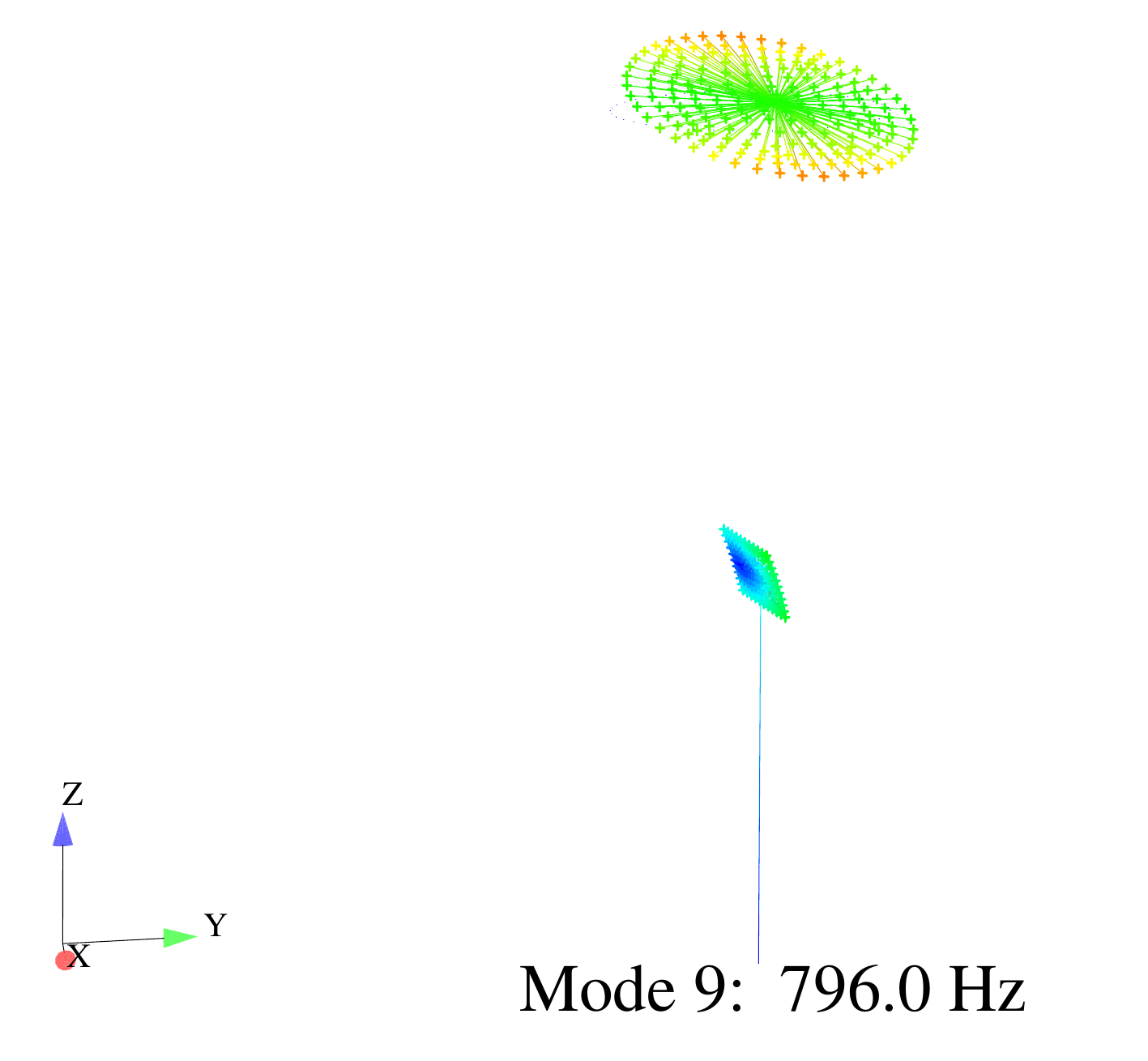
Figure 6.2 Modal Response of the Superelement.#