Example files on this page

• example input — Salinas_rtest/training/exampleproblem/randomvib/quad/vran1.inp

• Example Random Vibration Geometry — Salinas_rtest/training/exampleproblem/randomvib/quad/vtube.exo

9. Modal Random Vibration

Random vibration is a complex phenomenon. A random input with defined spectral characteristics is applied and the resulting power spectral response is computed. It may be complicated by having multiple inputs with statistically defined cross correlations. The modalranvib module in Sierra/SD performs this analysis using a linear superposition of normal modes. [1]

Input Deck and Exodus Requirements. The specification of the input for random vibration is complicated. The easiest way to perform this analysis is to copy an existing input specification and correct it for your specific model. The following sections will need attention.

The Exodus geometry specification is similar to other solutions.

Random load are often specified as an acceleration PSD, however an enforced acceleration cannot be used in the solution method for Sierra/SD. Instead of an enforced acceleration, a large concentrated mass may be inserted at the load point, and a Force applied to the mass. The load is then distributed to the structure through rigid elements (Rbars) or other means.

A nodeset must be identified on the load point, and node or side sets should be identified on any output points of interest. Be careful of nodal distribution factors other than 1!

As an example, we use the geometry shown in Figure 9.1. The load is applied to the mass on the left of the long tube. We clamp all dofs except the \(Y\) at the load point.

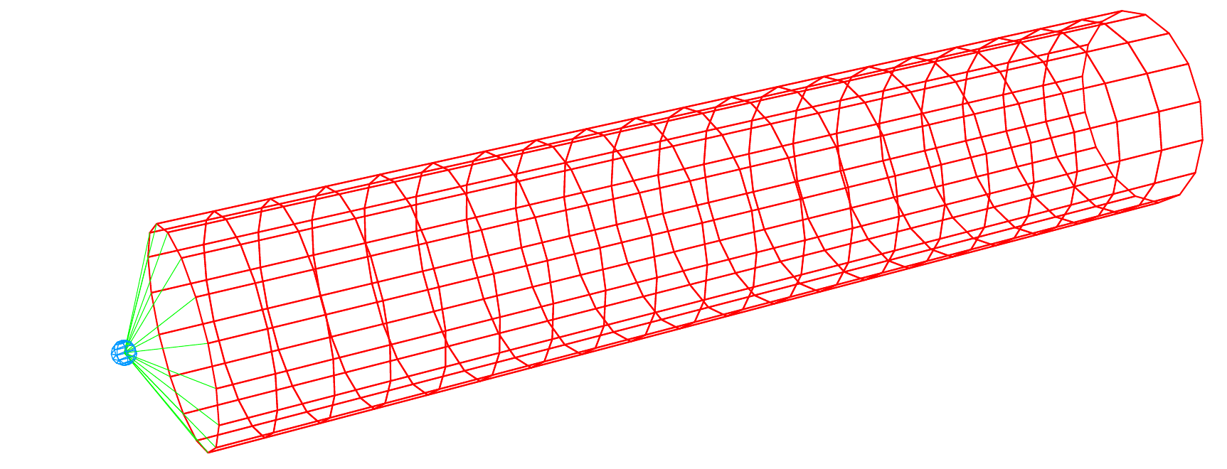
Figure 9.1 Example Random Vibration Geometry

9.1. Solution

The solution section is fairly straightforward, but note the following.

• While modalranvib can be performed in a single case solution, it is strongly suggested that a multicase solution approach be used. Most of the computational effort for a large model is typically consumed in computation of the normal modes. These calculations can be saved using the “restart” option. The calculations of the random vibration results from the modes cannot be restarted.

  Using multicase simplifies keeping track of the output files.

• There are two methods for computing these modes.

  • SVD.

    The default method is the more complete. It computes a vector representing the moment of the solution, and is recommended if detailed statistics on the statistical moments of von Mises stress are required.

  • noSVD.

    The noSVD version is faster. If many (hundreds) of modes are involved, then the noSVD version is significantly faster. The stress moments, \(M_2\) and \(M_4\), are also computed.

    \[ M_j = \int_{-\infty}^{\infty} \omega^j \sigma^2(\omega) d\,\omega \]

• Two parameters control culling of unwanted modes. The lfcutoff is used to control low frequency modes. It is important to set this to a large negative value if you wish to keep rigid body modes that may be important in the calculation of the autospectral response (see 9.4 below). On the other hand, these zero energy modes have no impact on stress, and are by default eliminated from the calculation.

  The keepmodes parameter can help reduce the number of modes used in the calculation. It truncates modes based on their activity for the given loads.

9.2. RanLoads

This section is the most complicated structure in Sierra/SD input files. A random input function, \(S_F(x,\omega)\) is Hermitian matrix valued, and depends on position, \(x\), and frequency. The matrix order \(n_f\) is the number of independent inputs.

If \(n_f=1\), then \(S_F\) is real valued, as illustrated in the full example of Section 9.3.

The random loads section of a multiple input case is shown below. In this case, loads are applied at three spatial locations as defined by the sideset and nodesets. The matrix-function (33) determines the correlation of these loads.

RANLOADS
  matrix=33   // defines a 3 by 3 matrix
  load=1      // associates next spatial distribution with row 1
    nodeset 11  // spatial distribution
      force= 0 1 0
  load=2      // associates next spatial distribution with row 2
    nodeset 22  // spatial distribution
      force= 1 1 0
  load=3
    sideset 3
      force=0 0 1
END

Most loads in Sierra/SD are described as a sum of spatial and temporal functions. For Random loads this is required, but in addition, the random loads are limited to having the same spatial variation for each row of the matrix. Thus, \(S_F\) has order \(3\), only three spatial functions are required. The spatial functions from the previous example are defined in nearly the same format as is used in a loads section. The balance of the definition is in the Matrix-Function section.

9.2.1. Matrix-Function

This section defines the dimension of the input and the frequency functions that define the temporal loading. For random vibration analysis, it must be of type Hermitian. Matrix functions may be symmetric if there is no cross correlation, as in a single input system. The matrix function will refer to one or more function definitions for the frequency content of each function.

Two different Matrix-Function sections are shown below. Both inputs describe the spectral input to a three input system. On the left, the inputs are completely uncorrelated (as there are no cross terms). The right example provides correlation between the inputs.

MATRIX-FUNCTION 33
   symmetry=symmetric
   dimension=3x3
   data 1,1
      real function 1
   data 2,2
      real function 1
   data 3,3
      real function 3
END

MATRIX-FUNCTION 33
   symmetry=Hermitian
   dimension=3x3
   data 1,1
      real function 1
   data 1,2
      real function 120
      imaginary function 121
   data 1,3
      imaginary function 131
   data 2,2
      real function 1
   data 2,3
      real function 220
      imaginary function 221
   data 3,3
      real function 3
END

As an aid in model verification, you may want to add nominalt to echo the value of the matrix at a single frequency.

9.2.2. Function

The function definition is standard. Note that the “loglog” type function was provided to help in the cases where the function is uses straight line interpolation in the log(frequency) and log(amplitude) domain (which is very common for power input). The units of the output of these functions is typically \(1/Hz\). It represents the frequency variation of the spectral density input.

9.2.3. Frequency

The frequency section is important for these reasons.

1. It provides the frequency band and step size over which the functions will be integrated. This affects the accuracy of the RMS calculations. Note however, that there is little penalty for increasing this quantity since the frequency integral is performed only once.

2. It is used to specify the output of frequency dependent transfer functions. For example, the acceleration PSD is defined as,

   \[ A(\omega) = H^\dagger(\omega) S_f(\omega) H(\omega). \]

   where \(H\) is the acceleration transfer function, and \(H^\dagger\) is the complex conjugate transpose.

   \[ H(\omega)=\sum_i \frac{-\omega^2} {\omega^2 -\omega_i^2 -2j\gamma_i\omega\omega_i} \]

   Thus, the output specification of the frequency block determines which of these output quantities will be written. Note that there is little point in outputting both displacement and acceleration as they only differ by a factor of \(\omega^4\).

   A special consideration should be given to the low frequency end of the frequency block. Rigid body modes are usually undamped, so a singularity may be introduced if zero is included in the frequency band.

9.2.4. Damping

Damping is important to this type analysis. Don’t forget it or leave it zero! All types of modal damping specifications are appropriate.

9.2.5. Output

Specification of Vrms is the only output specification that is honored for modal random vibration analysis. It triggers output of RMS values of stress, displacement and acceleration.

There are three values of RMS displacement – no results are output for rotational terms. The same is true for acceleration. Note that these quantities are not vectors. The RMS values indicate the most likely measurement of the square of the parameter, and includes the unique components of a Hermitian \(3\) by \(3\) matrix. It cannot be combined or transformed as vector.

9.2.6. Echo

The RMS values are typically written to the output Exodus file. They could also be written to the log file (or .rslt file) using the Vrms option. Some data is only available in the log file. If input is selected, then the log file will contain a list of those modes that were retained in the modal truncation together with the \(\Gamma_{qq}\) value for that mode. Modes for which the \(\Gamma_{qq}\) term are much smaller than other terms cannot contribute significantly to the total response.

9.3. Single Input Random Load Example

An example input for a single input random load is included, corresponding to the mesh shown in Figure 9.1.

The important components are summarized below:

• nmodes=55 in the eigen case of the SOLUTION block specifies that 55 modes will be computed. However, keepmodes=17 in the modalranvib case dictates that only the 17 most important modes will be retained in the calculation of RMS quantities.

• The ranloads block specifies that the load will be applied only to nodeset 12 (the concentrated mass), and that the force applied will be scaled by 1000 (the load mass). It also points to the matrix function 1 (matrix=1) for further input. The matrix-function section defines the load as a single input, and points to the PSD contained in function 1.

9.4. Verification of the Model

The obvious things come to mind in verifying the model for use in a random vibration analysis. First, ensure that the model is appropriate for eigen analysis. Mass properties and fundamental modes of vibration can be evaluated. Any rigid body modes should be near zero and not generate significant stress.

Second, the input PSD should be verified. Since the input cannot be provided as an enforced acceleration, it is typically specified as a load on a large mass. Examining the output acceleration at that degree of freedom should reproduce the input power spectrum. There are important issues that must be considered in evaluating the input PSD.

1. The rigid body modes of the system are critical to reproducing the input PSD. Typically, only one degree of freedom is left free on the load point, and that structure is loaded in that free direction. This corresponds to the action of a single axis shaker.

2. Rigid body modes are typically eliminated from the RMS stress calculation. This is done because these modes do not contribute to stress, and they may dominate the numerical solution, making it difficult to identify effects of other resonances. Further, one is often not interested in the rigid body mode contribution to the acceleration or displacement, except for the special case where the output PSD attempts to replicate the input. [2]

   Two factors can cause the rigid body modes to be removed from the calculation.

   • Rigid body modes are typically removed using a low frequency cutoff. This is easily managed using the lfcutoff parameter in the solution block. [3]

   • Any mode will be automatically eliminated if it is not a large contributor to the \(\Gamma_{qq}\) matrix. This is more difficult to manage, but is rare for rigid body modes.

3. As noted below, scaling can be a thorny issue.

When the force is applied directly to the system, without a large test mass, verification is similar, but care must be exercised on two counts.

1. It is usually best to eliminate all but the rigid body modes from the input verification because system resonances can have a large (and confusing) impact on the results. This can be done by setting the number of modes in the eigen solution to match the number of anticipated rigid body modes.

2. When there is a single input, the product of the output acceleration spectra and the square of the mass should equal the input power spectrum, (\(a^2 m^2 = S\)) provided that the force causes only a rigid body translation of the system. Rotations of the system confuse the verification. In other words, apply the load along the center of mass of the system or constrain out rotations in some manner.

Remember that the modal frequency response function can provide direct insight into the transfer functions.

A third verification is important for multiple inputs, where it can be easy to confuse the input to the \(S_F\) matrix. It can help to use the nominalt option in the solution block to provide an output of the matrix at some nominal frequency.

A word about scale factors and the Wtmass parameter is in order. To obtain the correct acceleration, the applied force must be multiplied by a scale factor. Note that the spatial term will be squared for terms on the diagonal of \(S_F\), so the units are still units of force (not those of force squared). For models with Wtmass=1, the input force is typically scaled by the product of the mass of the large mass times a factor of \(g\) to provide in input PSD in \(g^2/Hz\). For English units, where the Wtmass parameter is used to scale the mass from \(lbm\) to \(lbf\), that scale factor is already entered, and the force should be scaled only by the weight of the large mass. Some examples are provided below.

• Scaling SI units:

  In SI units, WTMASS=1. The acceleration of gravity is 9.8\(\,m/s\). Our nominal structure has a mass of 17 kg. To enforce acceleration, we add a 5000 kg mass and apply forces to it. We need to apply 1.5 g\(^2\)/Hz over the band.

  We establish the following.

  • A PSD function that applies \(1.5\) at all frequencies.

  • We determine that the force applied must be,

    \[ F = M_{\rm load} A = 5000 ( 9.8 ) \]

    The scale factor is 49,000.

• Scaling inches/pounds:

  For a model built in inches, with mass is specified in pounds, with WTMASS=0.002588 the mass has the proper units. Our nominal structure weighs 0.1 pounds, and to enforce acceleration, we add a \(100\) pound concentrated mass and apply forces to it. We have a complicated loading, with a maximum of \(200g^2\)/Hz at 1 KHz. Parameters used are the following.

  • Our PSD function matches our complex loading. It has a maximum of \(200\) at frequency \(1000\).

  • We determine the force to be applied.

    \[ F = M_{load} A = (100 \cdot 0.002588) ( 386.4 ) \]

    The scale factor is \(100\).

• Scaling English units:

  Our model is built in inches, and mass is specified in consistent units. We do not need to correct the mass units, so we have WTMASS=1. Our nominal structure has a mass of 258.8e-6 units, and to enforce acceleration, we add a \(0.250\) unit concentrated mass and apply forces to it. We have a complicated loading, with a maximum of 200g\(^2\)/Hz at 1 KHz. Parameters used are the following.

  • Our PSD function matches our complex loading. It has a maximum of 200 at frequency 1000.

  • We determine the force to be applied.

    \[ F = M_{load} A = (0.250) ( 386.4 ) \]

    Thus, our scale factor is set to 96.6.

9.5. What to do with the Results

The RMS values of displacement and acceleration can be very useful in determining what portions of the model may be experiencing large deformations or accelerations due to a random load. Unfortunately, RMS quantities are not vector quantities. They are difficult to display on a graphical representation of the data. One suggestion is that RMS displacement values be converted to an RMS radius, and spheres of that radius be plotted on the nodes of the structure.

Typically, RMS accelerations are not plotted on the structure. Such information may be useful for testing subcomponents. The full power spectra of acceleration is available at points specified as acceleration output in the frequency block, and may be used for test specification of subcomponents.

Root mean squared values of stress are more readily used, and may be displayed on the model any standard post-processor. Regions of high RMS stress indicate areas prone to failure either through instantaneously exceeding the yield stress, or through fatigue.

9.6. Limitations, Suggestions and Cautions

Must apply the loading directly to the model, you may not use enforced accelerations.

---

[1]

See Section 16 for a discussion of the loading for a random pressure loading applied on an extended surface. The modalranvib approach is more applicable to a loading on a handful of locations.

[2]

Sometimes we want to retain the rigid body modes for validation with experiment. This depends on the boundary conditions applied during the test.

[3]

The lfcutoff parameter must be used to retain the rigid body modes if you wish to replicate the input acceleration PSD. However, for numerical reasons, you should not normally retain rigid body modes when computing the RMS values of stress or displacement.