
Example files on this page
eigen input file — Salinas_rtest/training/exampleproblem/eigen/fixture/eigen.inp
Fixture Mesh — Salinas_rtest/training/exampleproblem/static/fixture/fixture.exo
modal transient simulation — Salinas_rtest/training/exampleproblem/transient/modaltrans/fixtureB/mtrans.inp
modalfrf input file — Salinas_rtest/training/exampleproblem/frf/modal/fixture/mfrf.inp
modalranvib input file — Salinas_rtest/training/exampleproblem/randomvib/fixture/rvib.inp
statics input file — Salinas_rtest/training/exampleproblem/static/fixture/static.inp
transient input file — Salinas_rtest/training/exampleproblem/transient/displacement/fixture/dtrans.inp
1. Solution Cases#
Sierra/SD supports different analysis types via solution cases. This section covers simple examples of several of the most common of these solution cases. Each of these input decks use the same “Fixture” mesh shown in Figure 1.1.
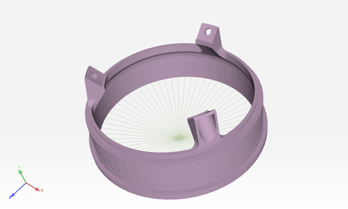
Figure 1.1 Fixture Mesh#
The sections of a Sierra/SD input file are described in the Sierra SD Users’ Guide. An input file has several common sections: solution, file (Exodus mesh), load(s), outputs, echo, block (one per element block in the input Exodus file) and material (one per unique material).
The statics input file has the common sections, and three optional sections: parameters, boundary and GDSW. The parameter Wtmass, typically \(1/(32.2 ft/s^2\) \(12 in/ft)\), is used so that for example densities may be specified in units of \(lbs/in^3\), as described in the Users’ Guide. Boundary conditions on a side set, or in this case a node set, are specified in the boundary section. The GDSW section indicates that the threshold on the relative residual norm be decreased from the default 1.e-6 if using the GDSW linear solver.
The eigen input file
requests that the twelve lowest frequency modes be computed. The eigen
norm parameter indicates that the mode shapes will be normalized in a
way that is convenient for visualization. The default normalization uses
the mass matrix. Here solver_tol has been further reduced to
\(1.e-10\).
The transient input file uses
the default Newmark method and has the total simulation time of 1/100
seconds. The load is specified by a tabulated Haversine pulse. The
history section indicates that the output quantities at each time step
and at the specified node sets only will be written to a different
Exodus output file with the suffix h. In this case the history file name
is fixture-out.h. The history file is \(20,000\) times smaller than the
ordinary output file. Finally, the restart option in the solution
section means that the file fixture-out.rslt_trans will be written. It
is possible to restart the simulation using this restart file, as
described in the Users’ Guide.
In a modal transient simulation, the transient problem is projected onto
the subspace spanned by the mode shapes of a user specified number of
the lowest frequency modes. Modal transient simulations are typically
much faster than direct transient analyses. The transient keyword has
been replaced by the modaltransient keyword. Also, a single input file
is used for both the initial eigenvalue problem (\(20\) modes), and the
following modal transient solution. This is called a multicase
solution. Another difference is that the plural loads section has been
replaced by a numbered load block to define a load that applies to the
transient solution, but not to the eigen solution.
Returning to the first solution case in the modal transient simulation, the eigenvalue problem, a shift is set to \(-1e+6\). Here the first eigenvalue is \(1e+8\). The eigenvalue problem is solved more efficiently and accurately if the shift is approximately \(-1\) times the lowest nonzero eigenvalue (flexible mode).
The modalfrf input file concerns the frequency response function. The frequency response function is used for example to confirm engineering assumptions about the frequency content of the accelerations.
Modal frequency response refers to using the mode shapes to diagonalize
the transfer function. A linear solver is not used to evaluate the
transfer function, but is used in solving the eigenvalue problem. The
function here describes the frequency dependent load, the Fourier
transform of the temporal load. The damping section supplies the
coefficient for mode proportional damping, \(C = \gamma M\). The
frequency block sets the spatial location and frequency range of the
load.
In the modal frequency response problem note that there is both a history section and a frequency section. The input file is for a multicase simulation. The history file section applies to the solution of the eigenvalue problem, and is ignored during the solution of the frequency response problem. The frequency response section is ignored during the solution of the eigenvalue problem, and applies only to the frequency response problem.
The modalranvib input file calculates the response of the to random vibration inputs. This solution has similarities to the modalfrf solution case and additionally requires a frequency dependent load definition. The outputs of this analysis are statistical properties of acceleration, velocity, displacement, and stress to the random vibration inputs. This case is covered in more detail in Modal Random Vibration.