Example files on this page

• input deck — Salinas_rtest/training/exampleproblem/eigen/buckling/ring20.inp

• Mesh File — Salinas_rtest/training/exampleproblem/eigen/buckling/ring20.exo

7.1.1. Linear Buckling

7.1.1.1. Shifted Eigenvalue

A challenging part of buckling analysis is determination of the shift parameter, which provides a convergence point for the solution. It should be chosen to be near the final solution, but not so near that the solver will fail due to a singularity. The eigenvalue problem involves the load dependent the material stiffness, \(K_g\). The system to be solved is,

\[ A = K_m - \lambda K_g. \]

The problem is solved using a shift invert strategy using ARPACK, where the operator is defined as,

\[ A = \left( K_m - \sigma K_g \right)^{-1} K_m \]

The buckling load must be multiplied by \(-\lambda\) to determine the critical buckling load.

Estimating a shift is easy if the solution has been found, but it is difficult until the loading is determined. Iteration may be necessary in many cases. First, note that the shift, \(\sigma\), will typically be a negative number for a structure in compression.

Consider the input deck and mesh shown below, with deformation as shown in Figure 7.3.

Figure 7.2 Mesh File

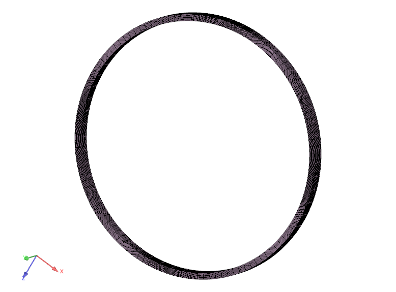
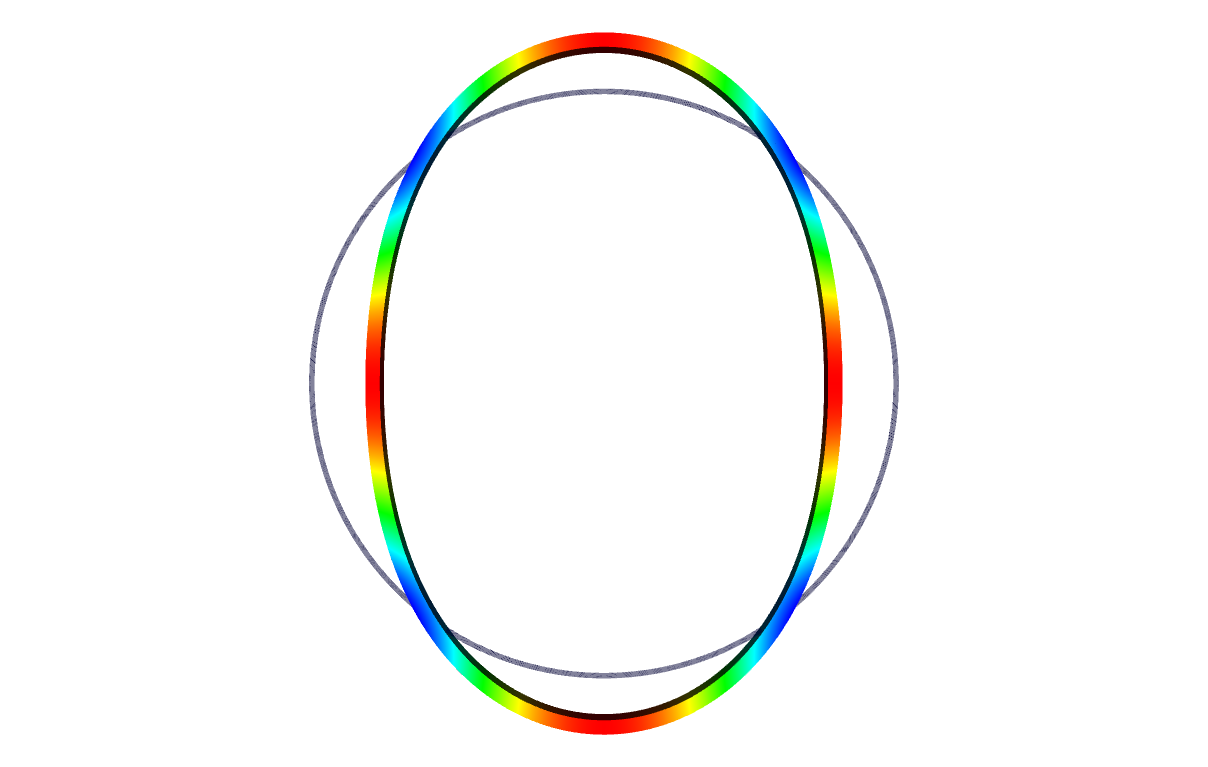
Figure 7.3 Deformation of ring model

Table 7.1 illustrates changes in behavior as a function of the shift parameter, \(\sigma\). As the shift value approaches the eigenvalue, the solution is found more readily. However, too large a shift results in an incorrect solution.

Table 7.1 Solution Dependence on Shift. A shift larger than the computed eigenvalue may generate solver issues (the matrix is negative), while shifts near zero have round off issues.

Shift	Eigenvalue	Time
-1000	-890.381	35
-500	-396.23	35
-400	-396.23	35
-396.23	-396.23	34
-380	-396.23	33
-200	-396.23	34
-100	-396.23	34
-50	-396.23	35
-10	-396.23	35
-1	-396.23	34
-1e-1	-396.232	35
-1e-2	-396.242	35
-1e-3	-394.775	35
-1e-4	-99.8013	35
-1e-5	-12.8036	35
-1e-6	-0.9631	35
-1e-8	-0.0105	35
1	fail	56
10	fail	53

Recommendations.

1. Get the sign of the shift correct. Objects in compression will require a negative shift.

2. If the magnitude of the eigenvalue is greater than the shift, reduce the shift to less than the eigenvalue.

3. You may want to evaluate a shift that is tiny relative to the eigenvalue. Generally, the eigenvalue should not be sensitive to the value of the shift.

4. The shift selected may impact the convergence of the linear solver. Generally a shift close to the eigenvalue leads to nearly singular linear system and may make the linear solver fail. A shift further from the solution may be easier on the linear solver, but may result in a poor convergence of the eigen solver.

7.1.1.2. Buckling Case Study

The pressure load at which the structure buckles is the buckling eigenvalue. This case study shows how to build confidence in a buckling result.

The critical eigenvalue is the mode of smallest magnitude. I prefer to compute \(10\) modes to check that I have computed the right mode. For example a model with symmetry has multiple mode shapes at the critical eigenvalue. Small eigenvalue residual norms boost my confidence in a result. The residual norms are shown in stdout. Improving the shift or reducing the linear solver tolerance may reduce the residual.

Suppose that initially pressure\(=-1\), shift\(=-100\) and solver_tol\(=1.e-6\), the eigenvalue is \(6.1637e4\), it has multiplicity two, and the residual norms are \(6e4\) and \(0.046\). The residual norms suggest that one of the approximate eigenvalues might be accurate. Given the eigenvalue we can improve the shift. The magnitude of shift should be of about the same as the magnitude as the eigenvalue but not too much larger. Shifting by \(-1.e4\) does not change the eigenvalue and decreases the residual to \(0.0036\). This gives me some confidence in the eigenvalue.

On the other hand if the initial pressure is \(-1.e-4\) with the same initial shift \(-100\) and solver_tol \(1.e-6\) then the eigenvalue is \(-2.84241e8\) and the residual\(=3300\) with product pressure eigenvalue \(=2.84241e4\). As this is the initial result nothing yet suggests that it’s wrong.

The first hint of a problem is that the smallest magnitude eigenvalue appears in the middle of the table of residual norms in row \(6\). It would be more encouraging for the smallest magnitude eigenvalue to be either at the top or the bottom of the table.

Here I will exercise my option to try a new shift instead of reducing the linear solver tolerance. The eigenvalue suggests the shift \(-1e8\).

With this shift the smallest eigenvalue is at the top of the table. The eigenvalue is \(6.16374e8\), the residual norm is \(.0017\), and the product pressure eigenvalue\(=-6.16374e4\). I have no confidence in the results due to the change in the product. However, the new shift reduced the residual by a factor of \(2e6\) lending credence to the new eigenvalue \(-6e4\). Decreasing the linear solver tolerance to \(1.e-8\) leads to similar conclusions.

It is a good practice in this case to try a different initial pressure. The predicted eigenvalue corresponding to pressure \(-1e4\) is \(-6\), suggesting the shift \(-1\). The smallest eigenvalue is in the first two rows. This is encouraging. It is also encouraging that the smallest residual is \(0.0029\). The product pressure eigenvalue \(=-6.16374e4\) has been reproduced.

Every simulation that I tried with shift \(-1/|pressure|\) reproduced the product pressure eigenvalue \(-6.16374e4\). The pressure load that will buckle the structure is the buckling eigenvalue \(6.16374e4\).