3.2.9. Mass Injection Boundary Condition

Incorporation of boundary layer development over an inflow surface can be achieved by the usage of a “mass injection” surface definition. For example, a quiescent pool fire notes entrainment over the pool surface due to vertical acceleration of the fire. Moreover, in crosswind applications that involve the release of a traceable species, a developing boundary layer interacts with the inlet. Fuego supports the ability to combine an inflow boundary that, in some cases, includes the presence of a wall. As will be discussed below, managing a “blowing” boundary condition from a wall is supported by the mass injection modeling approach. This boundary condition also provides the foundational implementation for the complementary fuel boundary condition that determines the mass flux of fuel given an incident heat loading. For more information regarding the pool boundary condition, please refer to Fuel Boundary Condition Submodel.

To begin the discussion of the mass injection boundary condition, Figure 3.2 outlines a typical exposed surface control volume for CVFEM. In this image, the near wall control volume is shaded with the degree-of-freedom (DOF) noted by the solid circular symbol. Triangles and diamonds depict surface- and volume-based integration points. The solid circle degree-of-freedom includes two elements, while the opposing node includes an inner element patch that is void of boundary contributions. The control volume shaded includes two boundary integration points. For a typical inflow, the known state entering the domain can be enforced either via a strong-form, i.e., Dirichlet, or a weak-form where advection and diffusion contributions are assembled to the control volume balance. In fact, the control volume approach allows for the natural integration-by-parts form for advection and diffusion. When using a Dirichlet approach, the specified value that is provided by the user prevails for the nodal DOF, and all other surface and volume contributions that may have been assembled during the iteration over elements are neglected.

The mass injection formulation provides the advective contribution, i.e., $\dot{m} \phi^{spec}$ , where $\dot{m}$ is the mass flow rate and $\phi^{spec}$ is the specified value that enters the domain, to the boundary node control volume. In the formulation, the mass flow rate is determined by the user-specified mass flux (units $mass/area/time$ ) and the integration point area. In Figure 3.2 two integration point contributions are made to the equation system. A diffusive contribution may also be added to the transport equation, if appropriate. For example, the momentum equation may compute a wall shear stress through a turbulent wall model and will have both an advective and diffusive contribution. Since the mass injection boundary condition is a mixture between an inflow and wall boundary condition, in some cases a Dirichlet condition due to the wall model specification parameters may prevail.

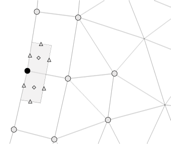
Fig. 3.2 Control volume definition for an exposed surface. The degree of freedom is noted by the dark circle; shading of the control volume is also indicated. Triangles and diamonds depict surface- and volume-based integration point locations.

A theoretical contributions due to the mass injection boundary condition are provided in the enumerated list below, while a condensed table that compares and contrasts the standard wall and mass injection boundary condition is presented in Table 3.5 and Table 3.6.

The continuity equation, which solves for the pressure DOF, assembles the computed integration point mass flow rate based on the user-specified mass flux and the integration point area.

The momentum equation, which solves for the velocity DOF, assembles $\dot{m}u_i$ . In this expression, $u_i$ is computed based on $\dot{m}/(\rho |A|)n_i$ , where $|A|$ is the integration point area magnitude and $n_i$ is the unit normal area component at the boundary integration point. The density used in this expression is based on user-specified conditions and follows the underlying material model evaluation. For example, if a mass injection temperature is specified, and the user activated an ideal gas law (uniform species), then density is computed based on the reference molecular weight, reference pressure, and wall injection temperature. The integrated viscous stress contribution is determined by the wall modeling approach. For a laminar-based configuration, the viscous stress tensor is integrated over the boundary surface and assembled to the wall-node equation system. For turbulent applications, the chosen turbulence modeling choices outlined in Wall Functions; Momentum dictate the wall shear stress closure. The effect of blowing on the wall friction velocity by default is assumed to be small and the standard wall boundary approach for the calculation of this variable is followed.

The transport equations including mixture fraction, mass fraction, soot-model transported equations, and user-defined progress variables assemble $\dot{m}\phi^{spec}$ to wall-node equation system, where $\phi^{sec}$ is the user-specified value. A zero diffusional flux is implied.

The enthalpy and conserved enthalpy equation set assembles $\dot{m} h^{MI}$ to wall-node equation system, where $h^{MI}$ is the derived enthalpy that is computed consistently with the property model and injection temperature specification. For example, $h^{MI}$ may be computed based on the injection temperature and species that the user specifies though a Cantera material property interface. For the diffusional contribution, the enthalpy supports a weak flux boundary condition for modeled turbulent wall treatments, and omits any contribution when a resolved laminar model set is active.

The turbulent kinetic energy equation, which solves for the modeled kinetic energy, assumes by default that the blowing contribution is small and is, therefore, neglected. The wall modeling approach outlined in Wall Functions; Momentum dictates the near-wall form for this DOF. For resolved modeling approaches, the user-specified value is used to enforce a Dirichlet condition. Models that require a normal distance to a wall include the mass injection surface in the determination of this variable. For the non-resolved model suite (in absence of a Dirichlet condition specification by the user), zero diffusion across the boundary surface is assumed.

The turbulence dissipation equation, which solves for the modeled turbulence dissipation, assumes by default that the blowing contribution is small and is, therefore, neglected. Like the turbulent kinetic energy and momentum equation, the wall modeling approach outlined Wall Functions; Momentum dictates the near-wall form for this DOF.

The elliptic relaxation equation, which is part of the $v^2-f$ model suite, applies a user-defined Dirichlet value at the wall.

The velocity-square equation, $\bar{v^2}$ , which is part of the $v^2-f$ model suite, also assumes by default that the blowing contribution is small and is, therefore, neglected. A weak boundary condition applying zero diffusion is implied.

Table 3.5 Wall details for supported equation sets.
Equation	Wall
	Advection	Diffusion
Continuity	Weak	n/a
Momentum	Zero	Strong (if wall-resolved), weak otherwise
Mixture-fraction	Zero	Weak (zero flux)
Mass-fraction	Zero	Weak (zero flux)
Soot-based	Zero	Weak (zero flux)
Progress variables	Zero	Weak (zero flux)
Enthalpy	Zero	Weak (if turbulent), Strong (if wall-resolved)
Conserved Enthalpy	Zero	Weak (zero-flux)
Turbulent KE	Zero	Zero (Weak or Strong)
Turbulence dissipation	Zero	Zero (Strong)
Elliptic Relaxation	Zero	Zero (Strong)
Velocity-square	Zero	Zero (Strong)

Table 3.6 Mass injection details for supported equation sets.
Equation	Mass Injection
	Advection	Diffusion
Continuity	Weak	n/a
Momentum	Weak, $\dot{m}u_i$	Weak
Mixture-fraction	$\dot{m}\phi^{spec}$	Weak (zero flux)
Mass-fraction	$\dot{m}\phi^{spec}$	Weak (zero flux)
Soot-based	$\dot{m}\phi^{spec}$	Weak (zero flux)
Progress variables	$\dot{m}\phi^{spec}$	Weak (zero flux)
Enthalpy	Weak, $\dot{m}h^{MI}$	Weak (if wall temperature is specified)
Conserved Enthalpy	Weak, $\dot{m}h^{MI}$	Weak (zero-flux)
Turbulent KE	Zero	Weak of Strong
Turbulence dissipation	Zero	Weak or Strong
Elliptic Relaxation	Zero	Zero (Strong)
Velocity-square	Zero	Zero (Strong)

3.2.9.1. Mass Blowing Correction for Turbulent Applications

In cases where mass injection is sufficiently high, the wall friction velocity must be modified. Fuego supports the following modified law of the wall form in such cases,

(3.236) $u^+ = {u_{\|} \over u_{\tau}} = { 1 \over \kappa } \ln \left(Ey^+\right) + K v^+$

The model constant $K$ is generally approximately ten, while the normalized blowing velocity is defined by ${v_{\perp} \over u_{\tau}}$ . For more information, the reader is referred to [42]. Note that model constant $E$ appearing above is generally modified to 8.166 for blowing walls and that stability of the nonlinear solve is reduced at high values of $v^+$ .