3.2.10. EDC Turbulent Combustion Model

The combustion submodel is Magnussen’s Eddy Dissipation Concept (EDC) and development details can be found in Magnussen, et al. [43], Magnussen [44], Byggsty{o}l and Magnussen [45], Magnussen [46], Lilleheie, et al. [47], and Gran and Magnussen [48].

3.2.10.1. Model Characteristics

The underlying assumption in the EDC model is that combustion in turbulent flows is controlled by turbulent mixing. The combustion model is an algebraic zone-type model and is influenced by local cell (control volume) values only. The model derivation assumes that the minimum cell dimension is large relative to the thickness of a flame (reaction zone) structure. This thickness varies with strain-rate, but the cell size should not be less than a few millimeters. The equations are not valid for laminar or near-laminar flow, but are based on fully developed turbulence arguments. The turbulent combustion model uses information from three sources: 1) thermochemistry, 2) species and state information from the cell values, and 3) turbulence kinetic energy and dissipation. From these data, the model creates source/sink terms for species equations and the energy equation (via radiative transport).

The model function is to provide an integral effect of combustion processes occurring within the control volume for the duration of a time-step. In this manner, reaction zone structures are not resolved, but the aggregate effect of turbulent combustion is modeled. To model the integral effect, two homogeneous zones are defined within each control volume for which there is combustion, as shown in Figure 3.3. The zones are termed the reaction zone (fine structures) and the surrounding zone. The size and mass exchange rate between these zones are influenced by the local turbulence properties and are the principal means by which turbulent fluctuations are accounted for within the model. The assumption that each zone is homogeneous is equivalent to assuming that the mixing within each zone is instantaneous. Since combustion occurs within (but is not limited to) the reaction zone, the assumptions for combustion correspond to those for a perfectly stirred reactor (PSR). Slower reactions can also occur in the surroundings, in which case, the assumptions for reaction in the surroundings are also consistent with PSR assumptions.

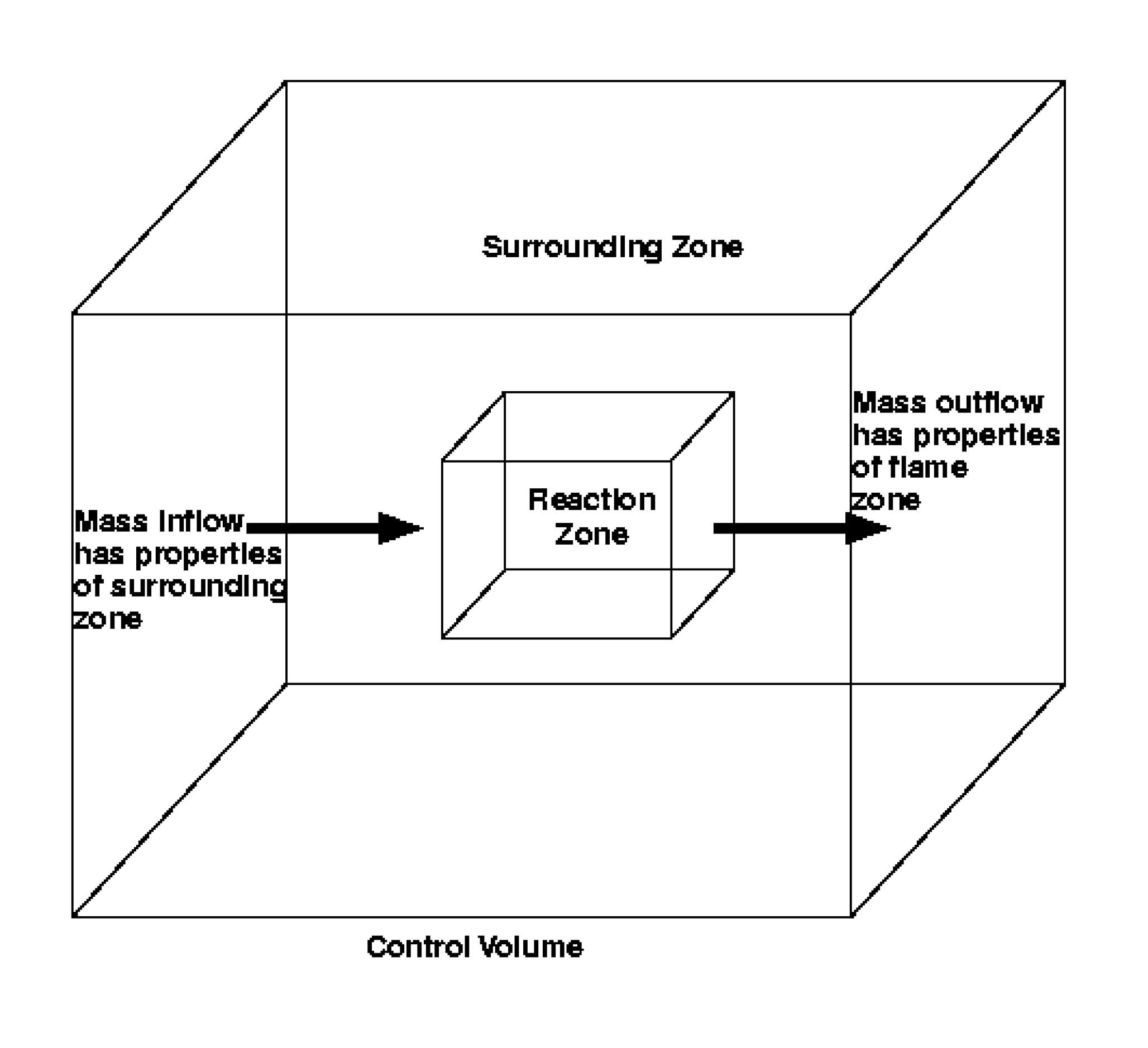
Model geometry for Magnussen's Eddy Dissipation Concept. The control volume is comprised of two zones; the properties of each zone are assumed to be adequately represented by a single set of values (i.e., lumped or perfectly stirred). The mass exchange between the zones is controlled by turbulent mixing. — Fig. 3.3 Model geometry for Magnussen’s Eddy Dissipation Concept. The control volume is comprised of two zones; the properties of each zone are assumed to be adequately represented by a single set of values (i.e., lumped or perfectly stirred). The mass exchange between the zones is controlled by turbulent mixing.

3.2.10.2. Physical Interpretation

Magnussen’s EDC model is derived to be a general combustion model for premixed to non-premixed scalar fields and for high to moderate turbulence levels. It is not intended to be used for laminar combustion. Magnussen’s physical interpretation of combustion is based on the concept that chemical reaction occurs in regions of the flow in which the dissipation of turbulent energy takes place, i.e., fine structure regions. These regions are concentrated in isolated volumes and represent a small fraction of the flow. The regions have characteristic dimensions that are of the Kolmogorov length scale in one or two dimensions, but not the third.

Fires are buoyant flows. Turbulent fires tend to be large, having base diameters above a meter. The turbulent length scales are large and the flow velocities are relatively slow, on the order of meters to tens of meters per second. (Still photographs of reaction zone structure within large fires can be found in Tieszen, et al. [49]). Therefore, turbulence levels tend to be moderate. Near the base of a fire, the combustion zone can be characterized as a continuous wrinkled flame sheet that appears to wrap around larger turbulent structures. The basic combustion mode is that of a strained diffusion flame with large surface area due to the turbulence. At higher elevations in the fire, turbulence levels increase and the character may change. Premixed combustion is possible as unburned products in the smoke are re-entrained into the fire. While Magnussen’s model was originally derived in terms of high turbulence levels resulting in fine structure regions (i.e., localized regions of high vorticity at dissipation scales), the model is appropriate for moderate turbulent intensities that occur in fires.

Figure 3.4 shows the physical geometry from which the combustion model will be derived for fires. Turbulence controls the reaction and surrounding volume fractions and fuel mass transport per unit volume. In general, turbulent momentum exchange processes result in scalar stirring at all length scales down to molecular mixing processes which are diffusion controlled. Without length scale information below the grid scale of the computation, it is impossible to correctly represent the interactions between all the relevant physical processes at their relevant length scales.

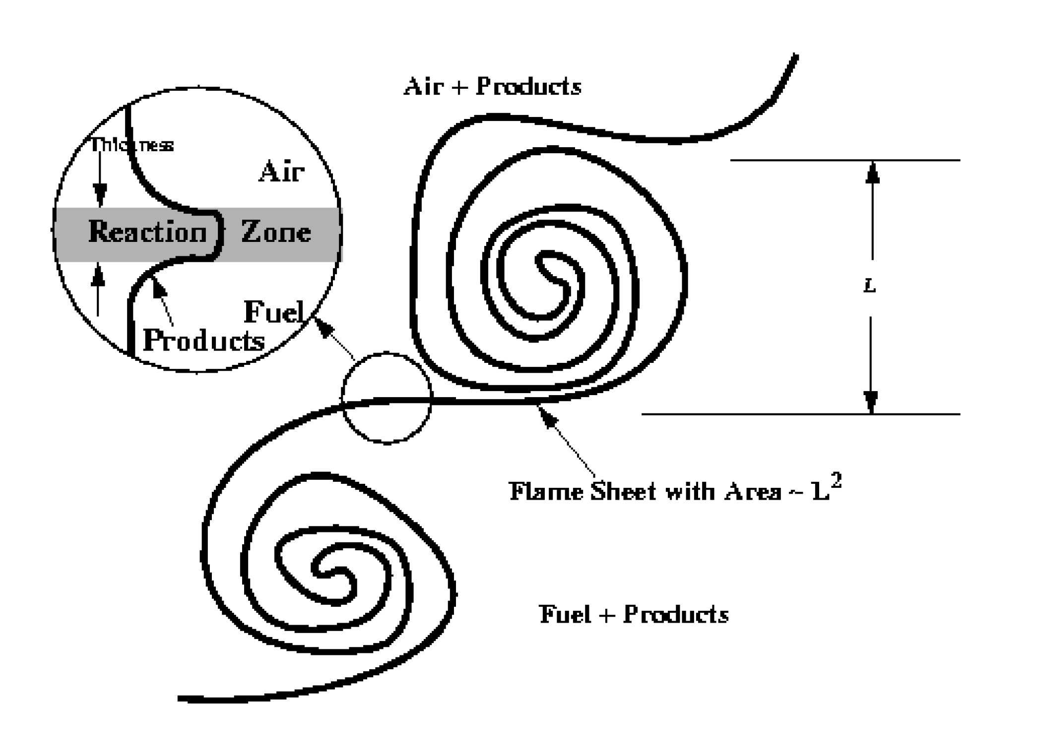
Assumed flame surface geometry. :math:`L` is the integral turbulent length scale. The reaction zone thickness is characterized by the Kolmogorov dissipative turbulent length scale, :math:`\eta`. — Fig. 3.4 Assumed flame surface geometry. $L$ is the integral turbulent length scale. The reaction zone thickness is characterized by the Kolmogorov dissipative turbulent length scale, $\eta$ .

Fig. 3.4 Assumed flame surface geometry. $L$ is the integral turbulent length scale. The reaction zone thickness is characterized by the Kolmogorov dissipative turbulent length scale, $\eta$ .

Magnussen’s EDC model attempts to represent the mixing processes that are most important to the overall heat release from combustion. It it based on the assumption that the overall heat release rate is controlled by the mass transport into the reaction zone. Therefore, considerable effort is made to model turbulent momentum processes that affect mass transport into the reaction zone. In the surrounding gases, turbulent mixing occurs with (in all likelihood) a similar vigor, however, its effect on the combustion rate is considered less important since the turbulence is not directly contributing to mass transport into the reaction zone. For this reason, there are two different levels of mixing assumptions made within the model.

With respect to Figure 3.3, the turbulence level in each control volume is taken into account in the consideration of the mass exchange between the reaction zone and the surrounding zone. However, within each zone, it is assumed that the properties are instantaneously homogeneous and uniform, i.e., perfectly stirred. This perfectly stirred assumption obviously over-predicts mixing within each zone for any real level of turbulence, and only begins to approximate reality at the highest levels of turbulence. On the other hand, the perfectly stirred assumption allows point calculations to be made in each zone for conveniently determining thermochemical properties. Without this assumption, it would be necessary to specify the gradients within each zone and integrate the specified gradients throughout the cell to obtain cell averaged property information. The approach here is to assume that over-predicting mixing within each zone via the perfectly stirred assumption has only a secondary effect on heat release rates within each cell.

3.2.10.3. Thermochemistry

Within the current strategy, chemical reaction can occur in both zones. However, in the simplest case, no reaction occurs within the surroundings due to the low temperature and unmixedness; all reaction occurs within the reaction zone. The notion of zones, perfect stirring within the zones, and type of chemistry involved are all independent assumptions, but have interrelated consequences. For example, finite-rate chemistry involving hundreds or thousands of species could be considered within the zones. From the perfectly stirred assumption within each zone, the finite-rate chemistry would be calculated as if it were occurring in a perfectly stirred reactor. In a real diffusion reaction, there are spatial variations in species concentrations for real turbulence levels so that the various chemical pathways, as well as heat, mass, and momentum transport, in a real strained diffusion flame can be quantitatively different than those calculated on the basis of perfect stirring. This effect is probably the strongest disadvantage of the perfectly stirred assumption. Only in the limit of infinitely-fast turbulent mixing does perfect stirring actually exist. In practice, the computation of detailed, finite-rate chemistry concurrently with a three-dimensional fluid mechanics calculation is expensive. Except in the limit where the turbulent strain rate is high enough that finite rate chemistry is warranted, it is adequate to use simpler descriptions of the chemistry. In the case of high strain rates, precalculation of the chemistry is usually done and the results tabulated in a look-up table to determine extinction limits.

For the current implementation, it is assumed that the chemistry can be represented as irreversible, “infinitely-fast” reactions that occur within each reactor. In classical combustion studies, the concept of “infinitely-fast” reactions is not usually invoked in the context of a perfectly stirred reactor. In the context of the current model, the meaning of an “infinitely-fast” reaction in the flame zone (a perfectly stirred reactor) is that the reactant stream entering the reaction zone is converted to products instantly as it enters the zone, and then the products are mixed instantly throughout the zone. The zone then reflects the thermodynamic properties of the combustion products at the adiabatic flame temperature for a given composition while the surrounding zone has the properties of reactants (and possibly previously combusted products) near the cell temperature.

In general, if the turbulent mass exchange rate between the zones (i.e. strain-rate) is sufficiently high that infinitely-fast chemistry assumptions do not apply, then finite-rate reactions within the perfectly stirred reactor can be used. Residence time scales that warrant finite-rate considerations tend to be at the sub-millisecond level. In the current implementation, the case of high turbulence levels leading to blow-out of a reactor is treated as a limits test. The test method is discussed in Limits Testing.

In principle, it is not necessary to assume irreversible chemistry within each zone. At long time scales (i.e., low turbulence levels), chemical equilibrium will result. The use of irreversible chemistry avoids the need to calculate the equilibrium state of the forward and reverse reactions for every combusting cell at every time step. For the current implementation, the time savings is deemed to be worth the cost in accuracy.

Regardless of the assumptions about chemistry employed in modeling the reaction zone, the actual reaction zones in a fire will very likely be similar to strained diffusion flames (wrinkled flame sheets wrapped into vortical structures). Perhaps higher in a fire with the re-entrainment of smoke, partially premixed combustion can occur. For diffusion reactions, combustion occurs within a region encompassing a stoichiometric surface between fuel and air. Therefore, the reaction zone is modeled as occurring with stoichiometric reactions. The reactants being transported into the reaction zone via turbulent mixing come from the surroundings zone and thus have the composition of the surroundings. There will be a limiting amount of one reactant if the combustion is to occur at off-stoichiometric conditions. The excess of the other reactant, prior products, and inerts do not participate in chemical reactions, but are transported in and out of the combustion zone by turbulent mixing. However, their presence affects the zone properties (for example, through their heat capacity).

Combustion products are transported into the surroundings at the same rate as the reactants are transported into the reaction zone (conservation of mass). However, the perfect stirring assumption for properties means that these products have uniform properties. In a diffusion reaction, products mix with fuel on one side of the reaction zone and air on the other. On the fuel side of the reaction zone, significant amounts of CO and soot can result from interaction between the inflowing fuel and outflowing products. The formation of CO is important not only from a toxic pollutant perspective but its formation results in significantly less heat release and lower temperatures. Given the limits of a two-zone model with perfect mixing within each zone, there is no simple way to model both stoichiometric combustion and the formation of CO on the fuel side of the reaction. In the current formulation, an ad-hoc approach is used in which combustion in the reaction zone is assumed to occur in sequential steps, each of which is irreversible and infinitely fast. The first step is stoichiometric oxidation of the fuel species to CO and ${\rm H}_2$ products. The second step is the oxidation of CO and ${\rm H}_2$ to ${\rm CO}_2$ and ${\rm H}_2{\rm O}$ provided there is excess ${\rm O}_2$ in the reactant stream. If the overall stoichiometry in the control volume is fuel rich, significant amounts of CO and ${\rm H}_2$ will be formed, while if it is lean only ${\rm CO}_2$ and ${\rm H}_2{\rm O}$ will be formed.

3.2.10.4. Chemical Mechanism

For an arbitrary CHNO fuel, the stoichiometric, irreversible reaction to CO and ${\rm H}_2$ products is given by

(3.237) ${\rm C}_m {\rm H}_n {\rm N}_p {\rm O}_q + \left({{m-q} \over 2}\right) {\rm O}_2 + \sum \left( \zeta_D \right){\rm Diluent} \quad \Rightarrow \left( m \right) {\rm CO} + \left( {n \over 2} \right) {\rm H}_2 + \left( {p \over 2} \right) {\rm N}_2 + \sum \left( \zeta_D \right){\rm Diluent} ,$

where $m$ , $n$ , $p$ , and $q$ are the numbers of carbon, hydrogen, nitrogen, and oxygen atoms within the fuel molecule, respectively, and the terms in parentheses are the stoichiometric coefficients.

The summation term for diluents includes all other species present in the reaction stream including nitrogen in air, combustion products in the surroundings from previous combustion processes, etc… Diluents, including the combustion products, are assumed to have no effect on the chemical reaction itself. However, diluents do have an effect on the temperature rise through their specific heats and the presence of products is used as an ignition criteria for the combustion model.

The assumption that combustion products act like diluents (i.e., have no effect on the reaction) is obviously a simplification. Product species include CO, ${\rm H}_2$ , ${\rm CO}_2$ , and ${\rm H}_2{\rm O}$ . The presence of CO and ${\rm H}_2$ in the reactant stream would affect equilibrium results; however, irreversible reactions have already been assumed in the model so the presence of these species does not represent an additional simplification. On the other hand, the presence of large amounts of ${\rm CO}_2$ and ${\rm H}_2{\rm O}$ in the reactant stream may reduce the amount of ${\rm O}_2$ consumed for a given amount of fuel due to partial oxidation of the products via the oxygen in the ${\rm CO}_2$ and ${\rm H}_2{\rm O}$ in an overall fuel rich environment. However, this effect is partially compensated since the extra ${\rm O}_2$ would be consumed by the second reaction.

The second reaction is the subsequent oxidation of CO and ${\rm H}_2$ to ${\rm CO}_2$ and ${\rm H}_2{\rm O}$ . This reaction oxidizes both the CO and ${\rm H}_2$ produced by the first reaction and any CO and ${\rm H}_2$ that passed through the first reaction as products (i.e., diluent). The reaction is given by

(3.238) $\left( m \right) {\rm CO} + \left( {n \over 2} \right) {\rm H}_2 + \left( {p \over 2} \right) {\rm N}_2 + \left( {m \over 2} + {n \over 4} \right) {\rm O}_2 + \sum \left( \zeta_d \right){\rm Diluent} \quad \Rightarrow \left( m \right) {\rm CO}_2 + \left( {n \over 2} \right) {\rm H}_2{\rm O} + \left( {p \over 2} \right) {\rm N}_2 + \sum \left( \zeta_d \right){\rm Diluent} .$

In the current implementation, soot is considered to be a trace species. As such, its mass and energetics are not considered part of the above chemical reactions. Soot has its own production terms and is considered to oxidize in proportion to the fuel oxidation in the first reaction. See the soot model in Soot Generation Model for Multicomponent Combustion for details.

3.2.10.5. Species Consumption/Production Limits

The reactants being transported into the reaction zone come from the surroundings and therefore have the same composition as the surroundings. As such, the reaction can only proceed within the limits of available fuel and oxygen from the reactant stream. For example, if there is insufficient oxygen in the reactant stream, then all of the oxygen will be consumed by Reaction 1, ((3.237)), and the excess fuel will be passed with products from Reaction 1 to Reaction 2, ((3.238)). Reaction 2 will not take place because all the oxygen was consumed in Reaction 1 (i.e., in both reactions, oxygen is limiting). If there is insufficient fuel in Reaction 1, then all the fuel will be consumed and excess oxygen will be passed to Reaction 2. Depending on the ratio of oxygen to CO and ${\rm H}_2$ , all the secondary fuels may be consumed or all the oxygen may be consumed.

To find the limiting mass, it is convenient to define an equivalence ratio. Equivalence ratios are normally defined in terms of molar ratios, but mass ratios yield the same result [50] and are preferred here since mass fractions are used in the transport equations.

(3.239) $\Phi = { \displaystyle{\left( {{Y_{fuel}} \over {Y_{oxy}}} \right)_{mix}} \over \displaystyle{\left( {{Y_{fuel}} \over {Y_{oxy}}} \right)_{stoic}}}$

The numerator is the ratio of the actual mass of fuel to oxygen in the reactant stream,

(3.240) $\left( {{Y_{fuel}} \over {Y_{oxy}}} \right)_{mix} = \left. {{\rm mass\ Fuel} \over {\rm mass\ Oxygen}} \right|_{\rm mix} .$

The denominator is determined for each reaction. Generically, the first and second reactions have the following form

(3.241) $\sum \left( \zeta_{fuel} \right){\rm Fuel} + \zeta_{O_2} O_2 + \sum \left( \zeta_D \right){\rm Diluent} \rightarrow \sum \left( \zeta_{prod} \right){\rm Product} + \sum \left( \zeta_D \right){\rm Diluent} ,$

where $\zeta$ are stoichiometric coefficients on a molar basis. The stoichiometric fuel to oxygen mass ratio is

(3.242) $\left. {{Y_{fuel}} \over {Y_{oxy}}} \right|_{stoic} = {{\sum W_{fuel} \left( \zeta_{fuel} \right)} \over {W_{O_2} \left( \zeta_{O_2} \right)}} ,$

where $W$ is a molecular weight. Specifically for the first reaction, the stoichiometric mass ratio of ${\rm C}_m{\rm H}_n{\rm N}_p{\rm O}_q$ to ${\rm O}_2$ is

(3.243) $\left. {{Y_{fuel}} \over {Y_{oxy}}} \right|_{stoic} = {{\left(12m+n+14p+16q\right)} \over {32 \left( \displaystyle{{m-q}\over 2}\right)}} .$

Therefore, the equivalence ratio for the first reaction which is based on carbon monoxide and hydrogen products is given by

(3.244) $\Phi_1 = \left({{Y_{fuel}} \over {Y_{oxy}}}\right) {{16 \left( m - q \right)} \over {\left(12m+n+14p+16q\right)}} ,$

and similarly, the equivalence ratio for the second reaction which is based on carbon dioxide and water products is given by

(3.245) $\Phi_2 = \left({{Y_{co}+Y_{h2}} \over {Y_{oxy}}}\right) {{16 \left( m + \displaystyle{n \over 2} \right)} \over {\left(28m+n\right)}} .$

If either equivalence ratio is greater than unity, then the mass of oxygen will be completely consumed by its reaction. If either equivalence ratio is less than unity, then the mass of fuel will be completely consumed by its reaction. If either equivalence ratio is unity, then the mass of fuel and oxygen will both be completely consumed by that reaction. Note that ${\rm C}_m{\rm H}_n{\rm N}_p{\rm O}_q$ is not a fuel in the second reaction because if there is any of this fuel left, all the oxygen was consumed in the first reaction. Therefore, under these conditions the second reaction cannot proceed due to lack of oxygen. Also note that the expression for $\Phi_2$ does not identify which secondary fuel, CO or ${\rm H}_2$ , is limiting.

In order to determine the limiting reactant mass in a multi-fuel (or multi-oxidant) system, a more general approach based on equivalence ratios is required. Consider the reaction $\zeta_A A + \zeta_B B \rightarrow \zeta_C C + \zeta_D D$ where $\zeta$ are stoichiometric coefficients. The stoichiometric mass ratio of reactant $B$ to $A$ is

(3.246) $\left. {{Y_B} \over {Y_A}} \right|_{stoic} = \left. {{{\rm mass}_B} \over {{\rm mass}_A}} \right|_{stoic} = {{W_B \zeta_B} \over {W_A \zeta_A}} .$

Further, $Y_A$ and $Y_B$ are the mass fractions of $A$ and $B$ in the mixture and

(3.247) ${{Y_B} \over {Y_A}} = \left. {{{\rm mass}\ B} \over {{\rm mass}\ A}} \right|_{mix} .$

The ratio of these quantities is an equivalence ratio; i.e., if

(3.248) ${{Y_B} \over {Y_A}} > {{W_B \zeta_B} \over {W_A \zeta_A}} ,$

then $A$ is the limiting reactant, else $B$ is the limiting reactant. However, this inequality can be usefully rearranged. If

(3.249) ${{Y_A} \over {W_A \zeta_A}} < {{Y_B} \over {W_B \zeta_B}} ,$

then $A$ is the limiting reactant. The same procedure can be shown to apply to reactions where there are more than two reactants; i.e., if

(3.250) ${{Y_A} \over {W_A \zeta_A}} < {{Y_B} \over {W_B \zeta_B}} < \cdots < {{Y_n} \over {W_n \zeta_n}} ,$

then $A$ is the limiting reactant of $n$ reactants. Therefore,

(3.251) ${\rm First\ Reactant\ Depleted} = \min_n \left({{Y_n} \over {W_n \zeta_n}}\right) .$

Note that the units of ${Y_n} / {W_n \zeta_n}$ are [ $({\rm mass}\ n)_{mix}/({\rm mass}\ n)_{stoic}$ ]/ $({\rm mass})_{mix}$ . Also note that diluents are not reactants and they are not depleted by the reaction. The $\min()$ function should only be applied to fuels and oxygen, not to all species.

To determine the change in mass fraction, $\Delta Y^m_k$ , of reactant species $k$ due to reaction $m$ , multiply the limiting mass expression by the stoichiometric mass of species $k$ :

(3.252) $\Delta Y^m_k = -W_k \zeta_k^m \min_n \left({{Y_n} \over {W_n \zeta_n}}\right)^{m} .$

This expression has units of [ $({\rm mass}\ k)_{stoic}/({\rm mass}\ n)_{stoic}$ ] $\times$ [ $({\rm mass}\ n)_{mix}/({\rm mass})_{mix}$ ]. Since $n$ is the limiting reactant, the expression within the second set of square brackets is the change in mass fraction of species $n$ due to reaction $m$ ; this is because the limiting species $n$ is completely used up in the reaction (i.e., the mass fraction of species $n$ goes to zero). The expression within the first set of square brackets modifies the change in mass fraction of species $n$ to yield the change in mass fraction of species $k$ due to reaction $m$ . The change in mass fraction of product species $k$ in reaction $m$ is similar but without the minus sign in the above expression.

Since the reactions are given priority, the “products” of Reaction 1 are the “reactants” of Reaction 2. The new mass fractions in the reactant stream for Reaction 2 are given by

(3.253) $\left(Y_k\right)_{\rm Reaction\ 2\ reactants} = \left(Y_k\right)_{\rm surr} \pm \Delta Y^{\rm Reaction\ 1}_k .$

As noted above, the sign of the second term, $\pm \Delta Y^{\rm Reaction\ 1}_k$ , is positive for products and negative for reactants. Similarly, the product composition from Reaction 2 is given by

(3.254) $\left(Y_k\right)_{\rm Reaction\ 2\ products} = \left(Y_k\right)_{\rm Reaction\ 2\ reactants} \pm \Delta Y^{\rm Reaction\ 2}_k .$

Here again the positive sign on the second term is used for products and negative sign is used for reactants. Since the reactions are assumed to occur infinitely fast, the product composition for Reaction 2 is the composition of the reaction zone,

(3.255) $\left(Y_k\right)_{\rm flame} = \left(Y_k\right)_{\rm Reaction\ 2\ products} .$

3.2.10.6. Conservation Laws

For convenience we restate the Favre-averaged species mass conservation equation, (3.106),

(3.256) $\int {{\partial \bar{\rho} \tilde{Y}_k} \over {\partial t}} {\rm d}V + \int \bar{\rho} \tilde{Y}_k \tilde{u}_j n_j {\rm d}S = \int \left( {{\mu} \over {\rm Sc}} + {{\mu_t} \over {{\rm Sc}_t}} \right) {{\partial \tilde{Y}_k} \over {\partial x_j}} n_j {\rm d}S + \int \overline{\dot{\omega}_k} {\rm d}V,$

where $\bar{\rho}$ is the time averaged density of the mixture, $\tilde{Y}_k$ is the Favre-averaged mass fraction of species $k$ , $\tilde{u}_i$ is the Favre-averaged velocity of the mixture, $\mu_t$ is the turbulent eddy viscosity, ${\rm Sc}_t$ is the turbulent Schmidt number, and $\overline{\dot{\omega}_k}$ is the time-averaged mass production rate of species $k$ per unit volume of the mixture. This equation is solved on a mesh, one control volume of which is shown in Figure 3.3. Within the control volume, the species $k$ mass consumption/production rate, $\dot{m}_{k,consumed/produced}=\overline{\dot{\omega}}_k V_{cell}$ , is determined by the EDC model, assuming that the mass transfer process into and out of the reaction zone from the surroundings (cf. Figure 3.3) can be represented as a steady process,

(3.257) $\left(\dot{m}_k\right)_{consumed/produced} = \left(\dot{m}_k\right)_{flame} - \left(\dot{m}_k\right)_{surr} .$

The mixture mass flow rate between the surroundings and the reaction zone is also assumed to be steady,

(3.258) $\left(\dot{m}\right)_{flame} = \left(\dot{m}\right)_{surr} .$

Combining these two expressions yields

(3.259) $\left(\dot{m}_k\right)_{consumed/produced} &= \left[ {{\left(\dot{m}_k\right)_{flame}} \over {\left(\dot{m}\right)_{flame}}} - {{\left(\dot{m}_k\right)_{surr}} \over {\left(\dot{m}\right)_{surr}}} \right] \left(\dot{m}\right)_{flame} &= \left[ \left(Y_k\right)_{flame} - \left(Y_k\right)_{surr} \right] \left(\dot{m}\right)_{flame} .$

It is convenient to normalize this equation with the mass of the control volume, or

(3.260) ${{\left(\dot{m}_k\right)_{consumed/produced}} \over {M_{cell}}} = \left[ \left(Y_k\right)_{flame} - \left(Y_k\right)_{surr} \right] {{\left(\dot{m}\right)_{flame}} \over {M_{cell}}} .$

The term in the brackets is a function of thermochemistry only and is specified by the chemical processes derived in the previous section. The second term, the normalized mass transfer rate, is a function of the turbulent mass exchange rate between the reaction zone and its surroundings. The derivation of this term is the subject of the next subsection.

3.2.10.7. Effect Of Turbulence On Combustion Rates

Magnussen derived the effect of turbulence on combustion rates in terms of high turbulence levels. The derivation here will be for moderate turbulence levels for the flame geometry shown in Figure 3.4. The derivation herein does not include proportionality constants. Rather, dimensional reasoning is used to establish the relationship between reaction zone surface area, volume, and mass transfer rates with respect to the prevailing turbulence levels. Constants of proportionality, taken from Magnussen’s original derivation, are added at the end.

Characteristic scales are needed for the mass transfer velocity into the reaction zone, the reaction zone surface area, and the reaction zone thickness. The mass transfer velocity into the reaction zone is a velocity appropriate to diffusional length scales that are being modified by the local strain field induced by the turbulent flow,

(3.261) ${\rm Mass\ Transfer\ Velocity} \propto \upsilon .$

An appropriate diffusional velocity is the Kolmogorov velocity, $\upsilon$ , which is characteristic of dissipative length scales (i.e., those in which the local strain field is being dissipated by diffusional effects). From Kolmogorov’s definition, $\upsilon$ is given by

(3.262) $\upsilon \equiv \left( \nu \epsilon \right)^{1/4} ,$

where $\nu$ is the molecular mixture kinematic viscosity (evaluated at the surrounding temperature), and $\epsilon$ is the rate of kinetic energy dissipation.

The reaction zone is characterized as a continuous flame sheet, highly wrinkled and wrapped around large eddies. The volume of a large eddy is characterized by

(3.263) ${\rm Volume}_{eddy} \propto L^3 ,$

where $L$ is the characteristic integral length scale of the turbulence. The reaction zone area is assumed to be proportional to both momentum and scalar influences. While all length scales of the turbulent cascade contribute to wrinkling and stretching the flame, it is assumed that large changes in surface area are associated with large length-scale fluctuations. Therefore, it is assumed that the square of the integral length scale is the most appropriate turbulent length scale for characterizing the reaction zone area.

Species concentrations also affect reaction zone area. Obviously, if no fuel is present, no reaction zone will be present regardless of level of turbulence present. The species influence are denoted by a function, $\chi$ , the rationale of which will be described later. Based on these arguments,

(3.264) ${\rm Area}_{flame} \propto \chi L^2 .$

To obtain property values for each zone in Figure 3.3, it is necessary to define the volume fractions of the reaction zone and surrounding zones. The reaction zone volume fraction is based on a reaction zone area and a reaction zone thickness. Since the reaction zone is a strain modified diffusional zone, its thickness is best modeled with a diffusional length scale that is characteristic of the turbulence-induced strain field. Thus the reaction zone thickness is proportional to the Kolmogorov scale, $\eta$ ,

(3.265) ${\rm Thickness}_{flame} \propto \eta .$

Kolmogorov’s definition of the diffusive length scale is

(3.266) $\eta \equiv \left({{\nu^3} \over \epsilon}\right)^{1/4} .$

Since this is a characteristic scale analysis, the molecular mixture viscosity is evaluated at the surrounding temperature. The actual reaction zone thickness will be larger due to the volumetric expansion (i.e., lower density) in the reaction zone.

Based on these characteristic scales from the assumed reaction zone geometry in Figure 3.4, expressions can be obtained for the mass transfer rate per total mass. The mass exchange rate into the reaction zone per unit eddy mass is given by

(3.267) ${{\dot{m}_{flame}} \over {M_{cell}}} = \left( {{\dot{m}_{flame}} \over {M_{eddy}}} \right) \left( {{M_{eddy}} \over {M_{cell}}} \right) .$

The first term on the right hand side is given by

(3.268) ${{\dot{m}_{flame}} \over {M_{eddy}}} = {{ \left({\rm Surrounding Density} \right) \left({\rm Flame Area} \right) \left({\rm Mass Transfer Velocity} \right) } \over { \left({\rm Eddy Density}\right) \left({\rm Eddy Volume}\right) }} .$

The interpretation of the second term on the right hand side depends upon filtering used (i.e., averaging over scales). For LES, the length scale of the eddy being modeled is proportional to the length scale of the grid. In this case, the size of the eddy and the grid are the same. Therefore, the second term is unity. In RANS modeling, the eddy is much larger than the grid, as is the reaction zone surface being modeled. For RANS, it is assumed that averaged over a sufficient number of eddies, the mass exchange rate into the reaction zone per unit eddy (first term) is uniformly distributed (i.e., independent of length scale) up to the integral length scales. In this case the second term is irrelevant and is assigned a value of unity. For example, for an integral scale eddy with a length scale ten times the grid, the mass transfer into the reaction zone (averaged over many eddies) would be ten times the value for an eddy with a length scale that is just the size of the grid.

Conservation of mass requires that the mass exchange rate into and out of the reaction zone be identical so the properties can be evaluated at the thermodynamic state of either the reactant stream (surroundings) or the product stream (reaction zone). For convenience, they will be defined in terms of the reactant stream temperature and mass fractions. Using the characteristic length and velocity scale arguments given above yields

(3.269) ${{\dot{m}_{flame}} \over {M_{cell}}} \propto {{\left(\rho_{surr}\right) \left(L^2 \chi\right) \left(\upsilon\right)} \over {\left(\rho_{cell}\right) \left(L^3 \right) }} = \chi {{\upsilon} \over L} {{\rho_{surr}} \over {\rho_{cell}}} .$

The standard integral scale estimate [10] of the rate of energy supply to diffusive scale eddies is

(3.270) $\epsilon \propto {{\rm Turbulent Kinetic Energy} \over {\rm Eddy Roll Over Time}} \propto {{{u'}^2} \over {L/{u'}}} = {{{u'}^3} \over {L}} .$

The turbulence kinetic energy is given as

(3.271) $k = {3\over2} {u'}^2 .$

Substituting and rearranging gives

(3.272) $L \propto {{k^{3/2}} \over \epsilon} .$

Ignoring the constant of proportionality and substituting the results into the definition for the Kolmogorov velocity gives

(3.273) $\upsilon \propto L \left({\epsilon \over k}\right) \left({{\nu \epsilon} \over {k^2}}\right)^{1/4} .$

Substituting gives the mass exchange rate into the reaction zone per control volume in terms of standard turbulence parameters,

(3.274) ${{\dot{m}_{flame}} \over {M_{cell}}} \propto \left({{\nu \epsilon} \over {k^2}}\right)^{1/4} \left({\epsilon \over k}\right) \chi {{\rho_{surr}} \over {\rho_{cell}}} .$

The function $\chi$ is a scalar correction to take into account species effects on the reaction zone area. The function is bounded between (0,1) with 1 representing optimal species concentrations which will maximize the reaction zone area and 0 representing prohibitive species concentrations which would prevent reaction zone formation. Two scalar properties are important, the reactant concentrations and the product concentration (which acts as an ignition source since ignition is not assumed). Therefore, the limiter is written as the product of two terms,

(3.275) $\chi = \chi_1 \chi_2 .$

The function $\chi_1$ is intended to take into account the effect of the reactant mass fractions on the reaction zone surface area. Since the reaction zone surface occurs at stoichiometric concentrations of fuel and oxygen in a diffusion flame, stoichiometric concentrations of reactants in a control volume will result in the largest reaction zone area (controlled by the turbulence levels). In this case, $\chi_1$ is unity. On the other hand, if either fuel or oxygen is zero within a control volume, then $\chi_1$ is zero. Between these extremes, a functional form is assumed which has the correct limiting properties. The function is given by

(3.276) $\chi_1 = {1 \over {\left( \displaystyle{{\hat{Y}_{oxy}+\hat{Y}_{prod}} \over {\hat{Y}_{min}+\hat{Y}_{prod}}} \right) \left( \displaystyle{{\hat{Y}_{fuel}+\hat{Y}_{prod}} \over {\hat{Y}_{min}+\hat{Y}_{prod}}} \right)}} ,$

where the normalized mass fractions are defined below.

Overall reaction stoichiometry is determined from the sum of Reactions 1 and 2 in the chemical reaction section ((3.237) and (3.238)). The overall reaction is

(3.277) ${\rm C}_m {\rm H}_n {\rm N}_p {\rm O}_q + \left(m+{{n-2q} \over 4}\right) {\rm O}_2 + \sum \left( \zeta_d \right){\rm Diluent} \quad \Rightarrow \left( m \right) {\rm CO}_2 + \left( {n \over 2} \right) {\rm H}_2{\rm O} + \left( {p \over 2} \right) {\rm N}_2 + \sum \left( \zeta_d \right){\rm Diluent}$

For the overall reaction, the mass ratio of oxygen to the mass ratio of fuel for stoichiometric reaction to ${\rm CO}_2$ and ${\rm H}_2{\rm O}$ is given by

(3.278) $S = \left( {{Y_{oxy}} \over {Y_{fuel}}}\right)_{Optimal} = \left( m + {n \over 4} - {q \over 2} \right) \left( {{32} \over {12m + n + 14p + 16q}} \right) .$

Since mass is conserved in the reaction, $1+S$ kilograms of product ( ${\rm CO}_2$ and ${\rm H}_2{\rm O}$ ) are produced for every kilogram of fuel consumed for a fuel/oxygen reaction. Note the mass of diluents, such as the nitrogen in the air does not change, as a result of the reaction. It is useful to produce normalized mass fractions based on the masses involved in the stoichiometric reaction.

(3.279) $\hat{Y}_{oxy} = {{Y_{oxy}} \over {S}} \qquad \hat{Y}_{prod} = {{Y_{co2}+Y_{h2o}} \over {1+S}} \qquad \hat{Y}_{fuel} = {{Y_{fuel}} \over {1}}$

Note that the sum of these terms does not equal unity but one minus the mass fraction of diluent in the mixture.

The actual reaction may involve the secondary fuels, so a more general expression is required for the stoichiometric mass ratio of oxygen to fuel (and is used in the Vulcan code).

(3.280) $S = { { {\rm SO2FU} \cdot Y_{fuel} + {\rm SO2CO} \cdot Y_{co} + {\rm SO2H2} \cdot Y_{h2} } \over { Y_{fuel} + Y_{co} + Y_{h2} } } ,$

(3.281) ${\rm SO2FU} = \left( m + {n \over 4} - {q \over 2} \right) \left( {{32} \over {12m + n + 14p + 16q}} \right) ,$

(3.282) ${\rm SO2CO} = {32 \over {2 \cdot 28}} ,$

(3.283) ${\rm SO2H2} = {32 \over {2 \cdot 2}} .$

The product mass fractions are adjusted for the mass of nitrogen that accompanies the oxygen in air – the nitrogen is treated as a product species. The normalized mass fractions are

(3.284) $\hat{Y}_{oxy} = {{Y_{oxy}} \over {S}} \qquad \hat{Y}_{prod} = {{3.39 Y_{co2}+3.92 Y_{h2o}} \over {1+ 4.29 S}} \qquad \hat{Y}_{fuel} = {{Y_{fuel}} \over {1}}$

where

(3.285) $\left. Y_{prod} \right|_{co2} = Y_{co2} \ \left( 1 + 3.76 {{MW_{n2}} \over {MW_{co2}}} \right) , \left. Y_{prod} \right|_{h2o} = Y_{h2o} \ \left( 1 + 1.88 {{MW_{n2}} \over {MW_{h2o}}} \right) ,$

The molar ratio of nitrogen to oxygen in air is 3.76 and the mass ratio is 3.29. The production mass fraction, $Y_{prod}$ , can be computed directly from the ${\rm CO}_2$ and ${\rm H}_2{\rm O}$ mass fractions as long as the only source of product species in the flow field comes directly from combustion. If there is injection of product species into the domain from a diluent stream or from an ambient concentration, then a transport equation should be solved for the product mass fraction (see Combustion Products Transport Equation).

Since combustion always occurs at a stoichiometric surface in a diffusion flame, there is a limiting reactant mass fraction in a fuel/oxygen mixture within the control volume unless the ratio is stoichiometric. The limiting reactant mass fraction is given by

(3.286) $\hat{Y}_{min} = \min \left( \hat{Y}_{fuel}, \hat{Y}_{oxy} \right) .$

The function $\chi_1$ can be seen to approach the correct limits most clearly if the mass fraction of products, $Y_{prod}$ , is set to zero. If the mixture is fuel lean, $\hat{Y}_{min}=\hat{Y}_{fuel}$ and $\chi_1$ is equal to the fuel to oxygen ratio which decreases to zero as the fuel mass fraction is decreased. If the mixture is fuel rich, $\hat{Y}_{min}=\hat{Y}_{oxy}$ and $\chi_1$ is equal to the oxygen to fuel ratio which decreases to zero as the fuel mass fraction is increased. At stoichiometric, $\chi_1$ is unity.

The function $\chi_2$ is intended to take into account the existence of reaction zone surface as a precondition for reaction zone surface propagation. A stoichiometric surface without reaction can exist in a flow field if there is no ignition source. An external source is required for ignition. However, once ignited, reaction zone propagation can be interpreted as new flame surface being ignited by existing adjacent reaction zone surface. A good indicator of existing flame surface is the presence of hot combustion products within the control volume and this fact is used to create the function $\chi_2$ .

The value of $\chi_2$ is zero if no combustion products are present. If the product mass fraction was uniformly distributed, then the probability of ignition would increase with the ratio of product mass fraction to reactant mass fraction. However, the combustion products are not uniformly distributed but concentrated around the reaction zones, thereby increasing the probability of propagation of reaction zone surface for a given product mass fraction. The assumed functional form of $\chi_2$ that has these characteristics is

(3.287) $\chi_2 = {{\left(\displaystyle{{\rm Existing Product Mass Fraction} \over {\rm Max Flame Volume}}\right)} \over {\left(\displaystyle{{\rm Max Possible Product Mass Fraction} \over {\rm Characteristic Product Volume}} \right)}}$

(3.288) $= \left( {{\rm Characteristic Product Volume} \over {\rm Max Flame Volume}} \right) \left( {{\rm Existing Product Mass Fraction } \over {\rm Max Possible Product Mass Fraction }} \right) . \nonumber$

The maximum volume of the reaction zone is the thickness times its area,

(3.289) $\gamma = {{\left( Area \cdot Thickness \right)_{flame}} \over {Volume_{eddy}}} \propto {{L^2 \eta} \over {L^3}} = {\eta \over L} .$

Using the definition for the Kolmogorov length scale and substituting the turbulence kinetic energy for length scale, $L$ , gives

(3.290) $\gamma \propto \left({{\nu \epsilon} \over {k^2}}\right)^{3/4} ,$

which is the maximum reaction zone volume per eddy volume. The value of $\gamma^{1/3}$ is bounded by one since the length scale ratio of the flame volume to eddy volume cannot be larger than one.

The characteristic product volume can be defined by assuming the majority of combustion products are held up within a distance corresponding to the Taylor microscale from the reaction zone surface,

(3.291) $\gamma_\lambda = {{\left( Area \cdot Thickness \right)_{prod}} \over {Volume_{eddy}}} \propto {{L^2 \lambda} \over {L^3}} = {\lambda \over L} .$

Note that this assumption is used only to establish an ignition probability. For actual property evaluation, it is assumed that the combustion products are well mixed with the surroundings. Taking the ratio of the volumes gives,

(3.292) ${{\gamma_\lambda} \over {\gamma}} \propto {\lambda \over \eta} .$

Using the standard definition of this ratio (Tennekes and Lumley [10]) gives,

(3.293) ${{\lambda} \over {\eta}} = {\rm Re}_L^{1/4} .$

The Reynolds number can be defined in terms of turbulent kinetic energy and its dissipation by,

(3.294) ${\rm Re}_L = {{k^2} \over {\nu \epsilon}} .$

Substituting gives,

(3.295) $\left({{\rm Characteristic Product Volume} \over {\rm Maximum Flame Volume}}\right) = \left( {1 \over {\gamma^{1/3}}} \right) .$

The existing product mass fraction is given by $Y_{prod}$ . The maximum possible product mass fraction is the sum of the existing products and the products that could be formed if all available reactants were to burn. Since combustion takes place at a stoichiometric surface, the limiting reactant mass fraction is given by $Y_{min}$ . Therefore, $\chi_2$ becomes

(3.296) $\chi_2 = \left( {1 \over {\gamma^{1/3}}} \right) \left( {{\hat{Y}_{prod}} \over {\hat{Y}_{prod} + \hat{Y}_{min}}} \right) .$

Functionally, $\chi_2$ can exceed unity but the product $\chi_1\chi_2$ is limited to the range (0,1). The function $\chi$ is now completely described in terms of species and turbulence properties.

Combining all previous results gives the following result for species consumption/production,

(3.297) ${{\left(\dot{m}_k\right)_{consumed/produced}} \over {M_{cell}}} \propto \left[ \left(Y_k\right)_{flame} - \left(Y_k\right)_{surr} \right] \left( \left({{\nu \epsilon} \over {k^2}}\right)^{1/4} \left( {\epsilon \over k} \right) \chi \left( {{\rho_{surr}} \over {\rho_{cell}}} \right) \right) ,$

where $\chi$ is defined above in terms of $\chi_1$ , $\chi_2$ .

The above derivation is intended to provide a physical interpretation to Magnussen’s EDC model for large fires typified by medium turbulence levels with diffusive combustion. Proportionality constants are needed to close the model. As always, constants can be tweaked for a given flow to produce the best result for that flow. However, we will use the constants as derived for more general flows (Ertesv{aa}g and Magnussen [51]). With these constants, the model equations match those from the KAMELEON-II-FIRE code (Holen et al. [52]).

Using these constants, the maximum reaction zone volume fraction is given by

(3.298) $\gamma = 9.7 \left( {{\nu \epsilon} \over {k^2}} \right)^{3/4} .$

Taking into account species limitations, the flame volume fraction is given by

(3.299) $\gamma\chi = 9.7 \left( {{\nu \epsilon} \over {k^2}} \right)^{3/4}\chi .$

The reaction rate of fuel is given by

(3.300) ${{\left(\dot{m}_k\right)_{consumed/produced}} \over {M_{cell}}} \propto \left[ \left(Y_k\right)_{flame} - \left(Y_k\right)_{surr} \right] \left( 23.6 \left({{\nu \epsilon} \over {k^2}}\right)^{1/4} \left( {\epsilon \over k} \right) \chi \left( {{\rho_{surr}} \over {\rho_{cell}}} \right)\chi_3 \right) .$

The additional scalar function, $\chi_3$ , at the end of (3.300) is multiplier on the combustion rate that Magnussen found necessary to maintain the mass transfer rate when the product concentration is high in premixed flames. Its necessity suggests that perhaps alternate scalings should be examined, but for consistency with the published model, it is implemented here as

(3.301) $\chi_3 = \min \left[ {{\hat{Y}_{prod} + \hat{Y}_{min}} \over {\hat{Y}_{min}}}, {1 \over {\gamma^{1/3}}} \right].$

3.2.10.8. Average Control Volume Properties

The volume and mass exchange process between the two zones is assumed to be constant over a time step. Consequently, cell averaged properties for the mean flow equations are a volume weighted sum of the properties in the two zones. Therefore, all control volume properties are given by

(3.302) $\phi_{cell} = {{\phi_{flame} V_{flame} + \phi_{surr} V_{surr}} \over { V_{cell} }} .$

The maximum volume fraction of the reaction zone, $\gamma$ , was determined previously from momentum considerations. The actual volume fraction is the maximum volume fraction times the scalar function, $\chi$ . The surroundings is the volume fraction that remains after the reaction zone volume has been removed. Therefore,

(3.303) $\phi_{cell} = \phi_{flame} \left( \gamma \chi \right) + \phi_{surr} \left( 1 - \gamma \chi \right) .$

Volume averaged properties given by (3.303) are desired. However, the estimates used to obtain $\gamma \chi$ (i.e., (3.298)) are based on uniform cell temperatures. Clearly, the flame zone will be hotter than the surroundings, so the volume fraction occupied by the flame will be larger than given by (3.303) (and the surroundings fraction smaller).

A first order non-isothermal estimate is made to account for flame volume fraction. This estimate assumes that the non-homogeneous density field does not affect the local turbulence field (or alternately, that dilatation cancels the baroclinic generation) such that isothermal, isotropic, homogeneous turbulence estimates for the turbulent kinetic energy, $k$ , and its dissipation, $\epsilon$ , hold. (This assumption is made in virtually all models by the necessity that the fundamental research to quantify the actual coupling has not been done.)

A mass balance then gives a first order estimate for the actual flame volume fraction at the flame temperature. The actual flame volume at the flame temperature is given by its isothermal estimate times the cell mean density (used to obtain the isothermal estimate) divided by the actual flame density.

Thus, (3.303) becomes,

(3.304) $\phi_{cell} = \phi_{flame} \left( \gamma \chi \right) {{\rho_{cell}} \over {\rho_{flame}}} + \phi_{surr} \left( 1 - \gamma \chi \right) {{\rho_{cell}} \over {\rho_{surr}}} .$

Where the mean density is given by

(3.305) $\rho_{cell} = \left[ { {\left( \gamma \chi \right)} \over {\rho_{flame}} } + { {\left(1 - \gamma \chi \right)} \over {\rho_{surr}} } \right]^{-1}.$

An interpretation of (3.304) and (3.305) is that $\gamma \chi$ , is intended as a non-isothermal volume estimate, which the mass weighted isothermal volume estimate happens to be the best available estimator until turbulence coupling in reacting flows can be elucidated. All cell averaged properties are given by (3.305). (3.303) is intended for clarification only.

3.2.10.9. Limits Testing

Parameters in the EDC model take on limiting values in the presence of piloting conditions and extinction conditions. The limits are discussing in the following subsections.

3.2.10.9.1. Ignition Criteria

Ignition will not occur in the above mechanism unless products are formed. An external ignition source (or pilot flame) is simulated by setting $\chi$ to be greater than zero (the product mass fraction is set to 0.2 times the maximum products that could be formed by the existing fuel in the current implementation) in a cell with fuel and oxygen present. This can be done on a cell by cell basis to represent point ignition sources, or in the whole domain if global ignition is required. If a pilot flame is to be simulated, the cells associated with it have $\chi$ set to be greater than zero for the duration of the calculation. If a transient ignition (e.g., spark) is to be simulated, the cells initially have $\chi$ set to be greater than zero. However, after a minimum temperature is reached within a cell, $T_{ign}$ (K) (a user input), $\chi$ is no longer specified but calculated from the species concentrations and turbulence levels as derived previously.

3.2.10.9.2. Extinction Criteria

Extinction occurs when $\chi = 0$ . This occurs automatically when the fuel and/or air is consumed. Local extinction can also be caused within a cell due to high turbulence levels. At high turbulence levels, the reaction zone can be appropriately modeled as a perfectly stirred reactor (PSR). A PSR blows out when the residence time is less than a minimum value for a given composition. The residence time, $\tau_{res}$ , in the reaction zone volume is given by

(3.306) $\tau_{res} = {{{\rm Volume}_{flame}} \over {{\rm Volume Flow Rate}_{flame}}} = {{\left( \displaystyle{{{\rm Volume}_{flame}} \over {{\rm Volume}_{cell}}} \right)} \over { \displaystyle{ \left( {{\dot{m}_{flame}} \over {\rho_{surr}}} \right) } \over { \left( \displaystyle{{M_{cell}} \over {\rho_{cell}}} \right) } } } .$

Simplifying gives

(3.307) $\tau_{res} = {{\chi \gamma} \over \displaystyle{\left({{\dot{m}_{flame}} \over {M_{cell}}}\right) {{\rho_{cell}} \over {\rho_{surr}}} } } .$

Substituting prior relations gives

(3.308) $\tau_{res} \propto {{\chi \left(\displaystyle{{\nu \epsilon} \over {k^2}}\right)^{3/4}} \over {\chi \left(\displaystyle{{\nu \epsilon} \over {k^2}}\right)^{1/4} \left(\displaystyle{\epsilon \over k}\right) }} .$

Simplifying and substituting Magnussen’s constant of proportionality gives

(3.309) $\tau_{res} = {1 \over {2.43}} \left( {\nu \over \epsilon} \right)^{1/2} .$

Comparison of the calculated residence time with a user input minimum residence time (based on pre-calculation using a PSR and appropriate chemistry) determines whether or not combustion is allowed to continue. If so, heat release is calculated as derived herein, and finite-rate effects are not considered. However, if the calculated residence time is below the minimum value, $\chi$ is set equal to zero which causes combustion to cease within a cell.

3.2.10.9.3. Laminar Values

As currently formulated, the model assumes the flow is fully turbulent and does not model laminar combustion. Minimum values for the reaction zone volume, $\gamma$ , and mass transport into the reaction zone per mass in the cell, $\dot{m}_{flame} / M_{cell}$ , are required in conditions with low turbulence levels to prevent singularities.

3.2.10.9.4. Scalar Limits

The mass fractions of fuel, air, and products must remain bounded (0,1). This requires that the consumption rate for the species with the limiting concentration times the time step must be less than or equal to the mass of species.

3.2.10.10. Cell Value Information Used By Model

The combustion model requires inputs from the transport equations for cell averaged variables at the start of a time step. These variables include pressure, $P_{th}$ (dynes/ ${\rm cm}^2$ ), species mass fractions $Y_i$ , density, $\rho_{cell}$ (g/ ${\rm cm}^3$ ), mixture molecular weight, $W_{mix}$ , (g/mole), turbulent kinetic energy, $k$ ( ${\rm cm}^2$ / ${\rm sec}^2$ ), dissipation of the turbulent kinetic energy, $\epsilon$ ( ${\rm cm}^2$ / ${\rm sec}^3$ ), mixture kinematic viscosity, $\nu$ ( ${\rm cm}^2$ /sec), individual (i.e., chemical plus sensible) enthalpies, $h_i$ (ergs/g), and mixture enthalpy, $h_{cell}$ (ergs/g).

3.2.10.11. Model Outputs

The two outputs of the combustion model are the species consumption rates and property estimates.

3.2.10.11.1. Species Consumption Estimates

Noting the general relation between cell averaged values and surrounding values, (3.303), the surrounding and cell mass fractions can be related to give

(3.310) $\left[ \left(Y_k\right)_{flame} - \left(Y_k\right)_{surr} \right] = {{ \left[ \left(Y_k\right)_{flame} - \left(Y_k\right)_{cell} \right] } \over { \left( 1 - \gamma \chi \right) }} .$

Substituting this result and the definition of $\tau_{res}$ into the species consumption/production rate gives the source term in the species transport equation, (3.256),

(3.311) $\overline{\dot{\omega}}_k = {{ \left[ \left(Y_k\right)_{flame} - \left(Y_k\right)_{cell} \right] } \over {\tau_{res}}} \left( {{ \gamma \chi} \over {1 - \gamma \chi}} \right) \chi_3 ,$

for the species mass production/consumption rate in a control volume. The subscript $k$ is understood to be for each species, ${\rm C}_m{\rm H}_n{\rm N}_p{\rm O}_q$ , ${\rm O}_2$ , ${\rm N}_2$ , CO, ${\rm H}_2$ , ${\rm CO}_2$ , ${\rm H}_2{\rm O}$ , and any diluents in the system.

3.2.10.11.2. Property Estimates

It is important in turbulent processes that nonlinear fluctuating quantities be appropriately represented. Properties for which nonlinear fluctuations are important include the radiative emissive power (proportional to the fourth power of temperature) and density.

To get the radiative emissive power, it is first necessary to get the temperature within each zone. This is accomplished by iterative estimate based on the species mass fractions within each zone. Since total (chemical plus sensible) enthalpy is used for each species, the total enthalpy per unit mass in the control volume does not change between the reaction zone or the surrounding zone. The partitioning of chemical and sensible enthalpy is different for the reaction and surrounding zone, but the specific total enthalpy is equal to the cell value defined at the beginning of each time step. (Note: this is not a statement of the energy equation, it is only a statement of property values within each zone and the cell. Obviously, the enthalpy does vary after radiation transport is allowed to occur and species are allowed to advect between cells at the end of the time step as governed by the energy equation).

The reaction zone temperature, $T_{flame}$ , is obtained from iterative solution of

(3.312) $h_{flame} = \left. \sum Y_k h_k \left( T \right) \right|_{flame} ,$

and the surrounding temperature, $T_{surr}$ , is obtained from iterative solution of

(3.313) $h_{surr} = \left. \sum Y_k h_k\left( T \right) \right|_{surr} .$

The average emissive power is given by

(3.314) $\sigma \overline{\alpha T^4}_{rad} = \sigma \bar{\alpha} \left( { T^4_{flame}\left(\gamma\chi \right) { {\bar{\rho}} \over {\rho_{flame}} } + T^4_{surr}\left(1-\gamma\chi \right) { {\bar{\rho}} \over {\rho_{surr}} } } \right) \qquad ({\rm ergs}/{\rm cm}^2{\rm-s}) .$

An important assumption implied by the form of (3.314) is that the turbulent fluctuations between the temperature and absorption coefficient are weakly correlated [7]. ( Note that the intent of the averaging form above is to volume-weight the emissive power from the flame and surrounding zones. This form implies that $\gamma\chi$ should be viewed as a mass fraction rather than a volume fraction as discussed for (3.302). )

The density of each zone can be calculated according to the perfect gas law. For the reaction zone volume, the density is

(3.315) $\rho_{flame} = {{P_{th} W_{flame}} \over {R T_{flame}}} ,$

where $R$ is the universal gas constant and $P_{th}$ is the constant thermodynamic pressure. For the surroundings, the density is

(3.316) $\rho_{surr} = {{P_{th} W_{surr}} \over {R T_{surr}}} .$

The soot model uses the temperatures, densities, and mass fractions of reaction zone and surroundings according to the above estimates.

3.2.10.12. Combustion Products Transport Equation

The product mass fraction represents the products formed by combustion ( $\mathrm{CO_2}$ and $\mathrm{H_2O}$ for hydrocarbon fuels, and $\mathrm{H_2O}$ for hydrogen fuel). If any of the product species are injected into the domain through either an initial condition or boundary condition to simulate a diluent stream or ambient concentration, their influence must be removed in order for the $\chi_2$ reaction limiter to function properly. A transport equation similar to (3.256) is used where the reaction rate is given by

(3.317) $\dot{\omega}_{prod} = 3.392 \dot{\omega}_{co2} + 3.924 \dot{\omega}_{h2o} .$

This transported product mass fraction can only be formed due to reaction within the domain and cannot be injected through either initial or boundary conditions. Therefore, the only boundary conditions that are required are at an outflow so that products may exit the domain, and a zero value at any surfaces where a species Dirichlet condition is applied. All of these cases are handled automatically so that nothing needs to be specified by the user.

Note that a pilot stream will be unable to ignite a flame when using this model. It will be treated as an inert diluent stream, so that the normal ignition model will be required to ignite the flame. This model in its current form should not be used for piloted flames.

Also note that if the only source of products in the simulation is combustion, then the product mass fraction can be computed directly from the local species mass fractions and solving this transport equation is unnecessary.

3.2.10.13. Chemical Equilibrium Models

The EDC combustion model uses a two-step chemical reaction, where the fuel species is consumed by the reaction in (3.237) to form $\mathrm{CO}$ and $\mathrm{H_2}$ , and then these intermediate species are consumed by the reaction in (3.238) to form $\mathrm{CO_2}$ and $\mathrm{H_2O}$ . If oxygen is present in excess, then none of the intermediate species will remain and only $\mathrm{CO_2}$ and $\mathrm{H_2O}$ will be produced. In reality, these reactions would not proceed to completion, but instead would reach an equilibrium where some of the intermediate species can persist. This can lead to a significantly different mixture composition and even a different mixture temperature than what the standard EDC model would predict, especially at higher temperatures.

Fuego includes two optional models that can include the effects of two independent chemical equilibrium reactions into the standard EDC model, to better predict high-temperature combustion species and temperatures.

3.2.10.13.1. $\mathrm{CO_2}$ Dissociation Model

At high temperatures, the equilibrium reaction

(3.318) $\mathrm{CO_2} \Leftrightarrow \mathrm{CO} + \frac{1}{2} \mathrm{O_2}$

becomes active to dissociate $\mathrm{CO_2}$ species back into $\mathrm{CO}$ and $\mathrm{O_2}$ , which has the effect to cool the gas mixture. Including the effects of this dissociation reaction will help to control nonphysically-high temperatures that might result otherwise.

This model will adjust the EDC-reacted mixture $(Y_k)_\mathrm{flame}$ in (3.311) to include the effects of equilibrium reaction (3.318). This equilibrium can be modeled by

(3.319) $K_p = \exp{\left(\frac{-\Delta G_T^o}{R_u T}\right)},$

where $R_u$ is the ideal gas constant, $T$ is the temperature at which the equilibrium is being calculated, $K_p$ is the equilibrium constant for this dissociation reaction, and $\Delta G_T^o$ is the standard-state Gibbs function change for this reaction. The equilibrium constant $K_p$ for (3.318) is defined as

(3.320) $K_p = \frac{ \left( \frac{P_\mathrm{CO}}{P^o} \right) \left( \frac{P_\mathrm{O_2}}{P^o} \right)^\frac{1}{2} }{ \left( \frac{P_\mathrm{CO_2}}{P^o} \right) },$

where $P_\mathrm{CO}$ , $P_\mathrm{O_2}$ , and $P_\mathrm{CO_2}$ are the partial pressures of $\mathrm{CO}$ , $\mathrm{O_2}$ , and $\mathrm{CO_2}$ , respectively, and $P^o$ is the reference pressure taken as $1\,atm$ . The standard-state Gibbs function change for this reaction can be evaluated in terms of the Gibbs function of formation for each species at temperature $T$ ,

(3.321) $\Delta G_T^o = \left( \bar{g}_{f,\mathrm{CO}}^o + \frac{1}{2} \bar{g}_{f,\mathrm{O_2}}^o - \bar{g}_{f,\mathrm{CO_2}}^o \right)_{T_\mathrm{ref}=T}.$

The partial pressure of species $k$ can be computed by $P_k = X_k P$ , where $P$ is the static pressure of the mixture and $X_k$ is the mole fraction of species $k$ , defined as $X_k = n_k / n_\mathrm{tot}$ with the total number of moles of all species being defined as $n_\mathrm{tot} = \sum\limits_i n_i$ . After making these substitutions and simplifying, the equilibrium equation that needs to be solved, written in terms of moles of each species in a fixed-mass volume, is

(3.322) $\frac{n_\mathrm{CO}\, n_\mathrm{O_2}^{1/2}}{n_\mathrm{CO_2}\, n_\mathrm{tot}^{1/2}} \left( \frac{P}{P^o} \right)^\frac{1}{2} = \exp{\left(\frac{-\Delta G_T^o}{R_u T}\right)}.$

Additional equations may be written to enforce conservation of $\mathrm{C}$ and $\mathrm{O}$ atoms within the reaction volume,

(3.323) $N_C = n_\mathrm{CO} + n_\mathrm{CO_2}$

(3.324) $N_O = 2\, n_\mathrm{CO_2} + n_\mathrm{CO} + 2\, n_\mathrm{O_2},$

where $N_C$ and $N_O$ are the fixed number of moles of carbon and oxygen atoms, respectively, during the equilibrium reaction. (3.322), (3.323), and (3.324) represent a system of three equations that can be solved for the three unknowns $n_\mathrm{CO_2}$ , $n_\mathrm{CO}$ , and $n_\mathrm{O_2}$ at the equilibrium state.

The numerical solution procedure begins by approximating the number of moles of each species from the reacted mixture mass fraction vector $Y_i$ as $n_i = Y_i / W_i$ , on a per-unit-mass-of-mixture basis. Eliminating $n_\mathrm{CO_2}$ and $n_\mathrm{O_2}$ from (3.322) yields a nonlinear equation that can be solved directly for $n_\mathrm{CO}$ from the fixed atom balances at a fixed temperature $T$ and pressure $P$ ,

(3.325) $n_\mathrm{CO}^2 \left(N_O - 2 N_C + n_\mathrm{CO}\right) - \left(\frac{P^o}{P}\right) \exp{\left(\frac{-2 \Delta G_T^o}{R_u T}\right)} \left(N_C - n_\mathrm{CO}\right)^2 \left(N_O + n_\mathrm{CO} + 2 \sum\limits_j^{N_\mathrm{inert}} n_j\right) = 0,$

where $\sum\limits_j^{N_\mathrm{inert}} n_j$ represents the summation of the number of moles of all species present in the mixture that do not participate directly in the equilibrium reaction, {it i.e.} all species except for $\mathrm{CO_2}$ , $\mathrm{CO}$ , and $\mathrm{O_2}$ .

A standard Newton’s method may be used to iteratively solve (3.325),

(3.326) $n_\mathrm{CO}^{n+1} = n_\mathrm{CO}^n - \frac{f(n_\mathrm{CO})}{f'(n_\mathrm{CO})},$

where the function $f(n_\mathrm{CO})$ is (3.325) and the derivative function $f'(n_\mathrm{CO})$ is

(3.327) $f'(n_\mathrm{CO}) = 2\, n_\mathrm{CO} \left(N_O - 2 N_C + n_\mathrm{CO}\right) + n_\mathrm{CO}^2 \\ - \left(\frac{P^o}{P}\right) \exp{\left(\frac{-2 \Delta G_T^o}{R_u T}\right)} \left[ \left(N_C - n_\mathrm{CO}\right)^2 - 2 \left(N_C - n_\mathrm{CO}\right) \left(N_O + n_\mathrm{CO} + 2 \sum\limits_j^{N_\mathrm{inert}} n_j\right) \right].$

Once this equation is solved for $n_\mathrm{CO}$ , then the following equations may be used to evaluate the remaining equilibrium species moles,

(3.328) $n_\mathrm{CO_2} = N_C - n_\mathrm{CO}$

(3.329) $n_\mathrm{O_2} = \frac{1}{2} \left( N_O - 2 N_C + n_\mathrm{CO} \right).$

With the new molar mixture defined for the equilibrium species, the mass fraction vector may be reconstructed by $Y_i = n_i W_i$ . This new mixture composition will result in a different temperature since the enthalpy is fixed. After the new temperature is evaluated, this entire procedure may be repeated iteratively until the mixture temperature converges to within a specified tolerance.

3.2.10.13.2. $\mathrm{H_2}$ Dissociation Model

Similar to the $\mathrm{CO_2}$ dissociation model described in \mathrm{CO_2} Dissociation Model, at high temperatures the equilibrium reaction

(3.330) $\mathrm{H_2} \Leftrightarrow 2\, \mathrm{H}$

becomes active to dissociate $\mathrm{H_2}$ species into $\mathrm{H}$ atoms, which has the effect to cool the gas mixture. Including the effects of this dissociation reaction in addition to the $\mathrm{CO_2}$ dissociation reaction will help to control nonphysically-high temperatures that might result otherwise.

This model will adjust the EDC-reacted mixture $(Y_k)_\mathrm{flame}$ in (3.311) to include the effects of equilibrium reaction (3.330). This equilibrium can be modeled by (3.319), with the equilibrium constant defined as

(3.331) $K_p = \frac{ \left( \frac{P_\mathrm{H}}{P^o} \right)^2 }{ \left( \frac{P_\mathrm{H_2}}{P^o} \right) },$

where $P_\mathrm{H}$ and $P_\mathrm{H_2}$ are the partial pressures of $\mathrm{H}$ and $\mathrm{H_2}$ , respectively. The standard-state Gibbs function change for this reaction can be evaluated in terms of the Gibbs function of formation for each species at temperature $T$ ,

(3.332) $\Delta G_T^o = \left( 2\, \bar{g}_{f,\mathrm{H}}^o - \bar{g}_{f,\mathrm{H_2}}^o \right)_{T_\mathrm{ref}=T}.$

Simplifying this equilibrium expression and writing it in terms of the number of moles of each species in a fixed-mass volume results in the equilibrium equation

(3.333) $\frac{n_\mathrm{H}^2}{n_\mathrm{H_2}\, n_\mathrm{tot}} \left( \frac{P}{P^o} \right) = \exp{\left(\frac{-\Delta G_T^o}{R_u T}\right)}.$

An additional equation may be written to enforce conservation of $\mathrm{H}$ atoms within the reaction volume,

(3.334) $N_H = n_\mathrm{H} + 2\, n_\mathrm{H_2},$

where $N_H$ is the fixed number of moles of hydrogen atoms during the equilibrium reaction. (3.333) and (3.334) represent a system of two equations that can be solved for the two unknowns $n_\mathrm{H_2}$ and $n_\mathrm{H}$ at the equilibrium state.

Similar to the $\mathrm{CO_2}$ dissociation model, the numerical solution procedure begins by approximating the number of moles of each species from the reacted mixture mass fraction vector $Y_i$ as $n_i = Y_i / W_i$ , on a per-unit-mass-of-mixture basis. Eliminating $n_\mathrm{H_2}$ from (3.333) yields a nonlinear equation that can be solved directly for $n_\mathrm{H}$ from the fixed atom balance at a fixed temperature $T$ and pressure $P$ ,

(3.335) $n_\mathrm{H}^2 - \frac{1}{4} \left(\frac{P^o}{P}\right) \exp{\left(\frac{- \Delta G_T^o}{R_u T}\right)} \left(N_H - n_\mathrm{h}\right) \left(N_H + n_\mathrm{H} + 2 \sum\limits_j^{N_\mathrm{inert}} n_j\right) = 0,$

where $\sum\limits_j^{N_\mathrm{inert}} n_j$ represents the summation of the number of moles of all species present in the mixture that do not participate directly in the equilibrium reaction, {it i.e.} all species except for $\mathrm{H_2}$ and $\mathrm{H}$ .

A standard Newton’s method may be used to iteratively solve (3.335),

(3.336) $n_\mathrm{H}^{n+1} = n_\mathrm{H}^n - \frac{f(n_\mathrm{H})}{f'(n_\mathrm{H})},$

where the function $f(n_\mathrm{H})$ is (3.335) and the derivative function $f'(n_\mathrm{H})$ is

(3.337) $f'(n_\mathrm{H}) = 2\, n_\mathrm{H} - \frac{1}{4} \left(\frac{P^o}{P}\right) \exp{\left(\frac{- \Delta G_T^o}{R_u T}\right)} \left[ \left(N_H - n_\mathrm{H}\right) - \left(N_H + n_\mathrm{H} + 2 \sum\limits_j^{N_\mathrm{inert}} n_j\right) \right].$

Once this equation is solved for $n_\mathrm{H}$ , then the following equations may be used to evaluate the remaining equilibrium species moles,

(3.338) $n_\mathrm{H_2} = \frac{1}{2} \left( N_H - n_\mathrm{H} \right)$