5.1.4. Radiative Flux BCs

This tutorial builds on the prior Convective Flux BCs tutorial and shows how to add a radiative flux boundary condition. This module has also been recorded in prior trainings and is available here or in the player below.

5.1.4.1. Problem Files

The files required for this tutorial can be downloaded here, or found at $SIERRA100/TF/Aria (where SIERRA100=/projects/sierra100 in a CEE environment, or your Sierra test distribution otherwise).

Aria input file

Mesh file

Training slides

5.1.4.2. Problem Domain/Mesh

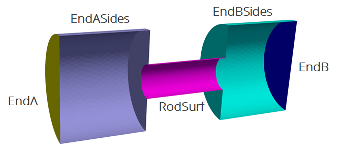
The geometry we will use for this tutorial is the same as the one used Basic Heat Conduction. It consists of three cylinders making a dumbbell shape, with three separate named blocks (ClampA, ClampB, and CenterRod). Blocks (volumetric sections in the mesh) are used in Aria to define different material properties, and can also be used to run post-processors on.

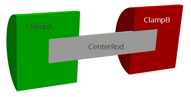
The problem also includes five separate named sidesets (EndA, EndB, EndASides, EndBSides, and RodSurf) applied on different surfaces of the mesh. Sidesets in aria are used to apply boundary conditions or do surface post-processing. Any surface not covered by a sideset will be treated as adiabatic, as will any sideset with no boundary condition applied to it.

The mesh file needed for this tutorial can be downloaded here, or it can be generated manually using the Cubit journal file shown in the Basic Heat Conduction tutorial.

5.1.4.3. Radiation in Aria

There are a few different ways to include thermal radiation into an Aria model, depending on what you are radiating to and what you are radiating through.

Simple Environment: For radiative exchange with a simple environment with a known or pre-computed view factor one can apply a simple flux model where $q = \sigma \epsilon F (T^4 - T_{ref}^4)$ . In this approach you would prescribe values or models for $\epsilon$ , $F$ , and $T_{ref}$ .
Enclosure Radiation: For radiative exchange between surfaces in your model through an optically thin media you can use the enclosure radiation capability. This will calculate view factors between all faces in the enclosure and do a radiosity solve to determine radiative fluxes. The enclosure can be closed or open to a prescribed environment. This option can be expensive for large enclosures since the cost scales with $N^2$ where $N$ is the number of faces in the enclosure.
Participating Media Radiation: When the media through which you are radiating is optically thick (absorbs and re-emits instead of being mostly transparent) then you can use a meshed enclosure to couple Aria and PMR to do a discrete ordinate solve of the radiative transport equation.

This tutorial will use the simple environment approach to add radiation to the outer surfaces of the dumbbell geometry.

5.1.4.4. Adding a Radiative BC

Scope: Aria Region

First, we will add a new mesh group to make applying the radiative boundary conditions easier. The mesh group rad_surfs will include all surfaces except the two on the ends.

Mesh Group rad_surfs = all_surfaces - EndA - EndB
BC Flux for Energy on rad_surfs = Generalized_Rad T_ref = 250

Since we are applying a constant value for $T_{ref}$ we can use the Generalized_Rad boundary condition.

5.1.4.5. Post-process Flux

Scope: Aria Region

By default, the ENERGY_FLUX is the sum of all the applied flux BCs. If we want to postprocessor separate contributions from the two flux models we have (convection and radiation) we can pass the model name to the postprocessor.

Postprocess value of expression energy_flux on RodSurf Model Generalized_Nat_Conv as ConvFlux
Postprocess value of expression energy_flux on RodSurf Model Generalized_Rad as RadFlux

We will now get a new RadFlux nodal field that is just the radiative flux contribution. To be able to see this fields, we need to also add it to the results output block.

Begin Results Output AriaOutput
    Title Aria: Transient Training Model
    Database Name = heat_cond.e
    At Step 0 Interval = 5
    Nodal Variables = Solution->Temperature as T
    Nodal Variables = ConvFlux
    Nodal Variables = HeatFlux
    Nodal Variables = RadFlux

    Global Variables = FluxA
    Global Variables = FluxB
    Global Variables = ClampConvLoss
    Global Variables = RodConvLoss
End

5.1.4.6. Running Aria

Once you have finished setting up the input file, you are ready to run Aria. From a CEE unix environment, you can load the sierra module to access the latest release of Aria to run it on your local machine. To run it on 4 processors, you could use

$ module load sierra
$ launch -n 4 aria -i heat_cond_session4.i

5.1.4.7. Viewing the Results

From a CEE unix environment with graphics, you can launch paraview using

$ module load viz
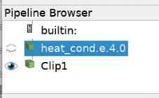
$ paraview heat_cond.e.4.0

Or if you have installed Paraview locally, you can launch it and select the exodus file from the appropriate file opening menu.

Once you have loaded it, you need to select which variables to show then click Apply.

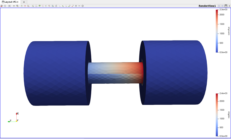
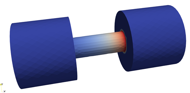
To show the convective flux field (RadFlux) on the center rod, you can

Go to the last time step

Select the RadFlux variable to show

Rescale the color scale if needed

The result shows how the radiative flux varies across the center rod

To compare the radiative and convective flux

Clip the domain and click Apply (with the default clipping normal of 1 0 0)

Re-select the original data set in the pipeline browser

Clip the domain again, with the clipping normal set to -1 0 0 and click Apply

Choose RadFlux to show on the first clipped data set and ConvFlux on the second