5.1.2. Materials and Flux BCs
This tutorial builds on the prior Basic Heat Conduction tutorial and shows how to add a more complicated material and set flux boundary conditions. This module has also been recorded in prior trainings and is available here or in the player below.
5.1.2.1. Problem Files
The files required for this tutorial can be downloaded here, or found at $SIERRA100/TF/Aria (where SIERRA100=/projects/sierra100 in a CEE environment, or your Sierra test distribution otherwise).
5.1.2.2. Problem Domain/Mesh
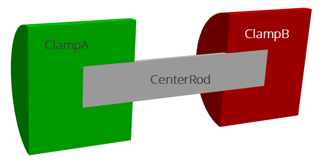
The geometry we will use for this tutorial is the same as the one used Basic Heat Conduction. It consists of three cylinders making a dumbbell shape, with three separate named blocks (ClampA, ClampB, and CenterRod). Blocks (volumetric sections in the mesh) are used in Aria to define different material properties, and can also be used to run post-processors on.
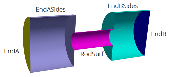
The problem also includes five separate named sidesets (EndA, EndB, EndASides, EndBSides, and RodSurf) applied on different surfaces of the mesh. Sidesets in aria are used to apply boundary conditions or do surface post-processing. Any surface not covered by a sideset will be treated as adiabatic, as will any sideset with no boundary condition applied to it.
The mesh file needed for this tutorial can be downloaded here, or it can be generated manually using the Cubit journal file shown in the Basic Heat Conduction tutorial.
5.1.2.3. Defining Complex Materials
Scope: Domain
In the prior tutorial we used a single material with constant properties for all blocks in the mesh. For this example we will add a second material - 304 stainless steel - and use it on one of the blocks. This material will use temperature-dependent properties for specific heat and thermal conductivity. For more information on material definition refer to Material Properties.
Begin Aria Material ss304
  Density              = Constant value = 8000
  Specific Heat        = Polynomial Variable=Temperature order=1 C0=500 C1=0.1
  Thermal Conductivity = User_Function name=ssteel_k_function X=temperature
  Heat Conduction      = Generalized
End   Aria Material ss304

Begin Definition for Function ssteel_k_function
  Type is Piecewise Linear
  Begin Values
    #T (K)  k (W/mK)
    100    10
    500    20
  End Values
End   Definition for Function ssteel_k_function
We used a user function to define the thermal conductivity from a table of values at different temperatures. Since it is a Piecewise Linear table, the value for conductivity will be interpolated linearly between the points of the table.
We also used a polynomial model to define a linear specific heat ( ) - we could also have used a string function to get the same result
Specific Heat = Scalar_String_Function f = "500 + 0.1*temperature"
For a complete list of the available models to use for a given property, you can refer to the Material Properties section of the user manual. For example, to see all available models for specific heat you could go to the specific heat section.
5.1.2.4. Applying the new Material
Scope: Domain
To apply the new stainless steel material to one of the blocks, we must edit the Finite Element Model block where mesh blocks were previously all assigned to use the aluminum material.
Begin Finite Element Model FEModel
    Database Name = mesh.g
    Use Material aluminum for ClampA ClampB
    Use Material ss304 for CenterRod
End   Finite Element Model FEModel
5.1.2.5. Updating Boundary Conditions
Scope: Aria Region
In the prior tutorial we used Dirichlet boundary conditions - specified temperature - on both ends of the domain. For this case we will change one of those boundary conditions to a specified time-varying flux. Delete the Dirichlet BC from EndB and replace it with the following flux BC:
BC Flux for Energy on EndB = scalar_string_function f = "-5e4*sin(t/300)"
Note
The sign convention for flux BCs in Aria is that positive = outflux.
To see all the available boundary condition models, you can use the boundary condition section in the user manual.
5.1.2.6. Post-process Flux
Scope: Aria Region
Aria supports a large number of different postprocessors. Postprocessors can be used to calculate spatially varying fields of material properties or intermediate calculations, or can be used to do reductions (integral, average, min, max, etc) to produce global variables. In this case, we will use the integrated_flux postprocessor to calculate the total flux on both ends of the domain.
Postprocess integrated_flux of equation energy on EndA as FluxA
Postprocess integrated_flux of equation energy on EndB as FluxB
This will produce two global variables - FluxA and FluxB. These will be printed to the log file, and can also be output to a heartbeat file (a text file) or included in the regular exodus output. For this example we will just add them to the existing exodus output file.
Begin Results Output AriaOutput
    Title Aria: Transient Training Model
    Database Name = heat_cond.e
    At Step 0 Interval = 5
    Nodal Variables = Solution->Temperature as T

    Global Variables = FluxA
    Global Variables = FluxB
End
5.1.2.7. Running Aria
Once you have finished setting up the input file, you are ready to run Aria. From a CEE unix environment, you can load the sierra module to access the latest release of Aria to run it on your local machine. To run it on 4 processors, you could use
$ module load sierra
$ launch -n 4 aria -i heat_cond_session2.i
5.1.2.8. Viewing the Results
From a CEE unix environment with graphics, you can launch paraview using
$ module load viz
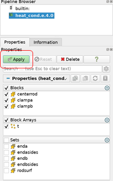
$ paraview heat_cond.e.4.0
Or if you have installed Paraview locally, you can launch it and select the exodus file from the appropriate file opening menu.
Once you have loaded it, you need to select which variables to show then click “Apply”
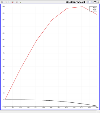
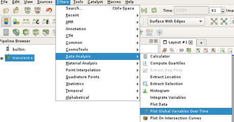
To plot the global variables (fluxes on the two ends of the domain)
Go to the Filters menu and select “Data Analysis” then “Plot Global Variables Over Time”
Click “Apply” to generate the plots
The result shows how the flux varies over time