5.1.1. Basic Heat Conduction
This tutorial shows how to set up a basic transient heat conduction problem in Aria. This module has also been recorded in prior trainings and is available here or in the player below.
5.1.1.1. Problem Files
The files required for this tutorial can be downloaded here, or found at $SIERRA100/TF/Aria (where SIERRA100=/projects/sierra100 in a CEE environment, or your Sierra test distribution otherwise).
5.1.1.2. Problem Domain/Mesh
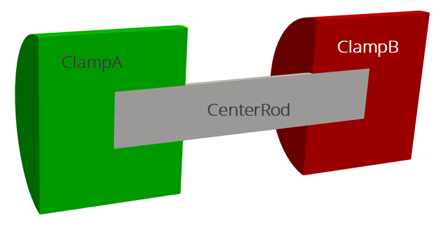
The geometry we will use for this demonstration consists of three cylinders making a dumbbell shape, with three separate named blocks (ClampA, ClampB, and CenterRod). Blocks (volumetric sections in the mesh) are used in Aria to define different material properties, and can also be used to run post-processors on.
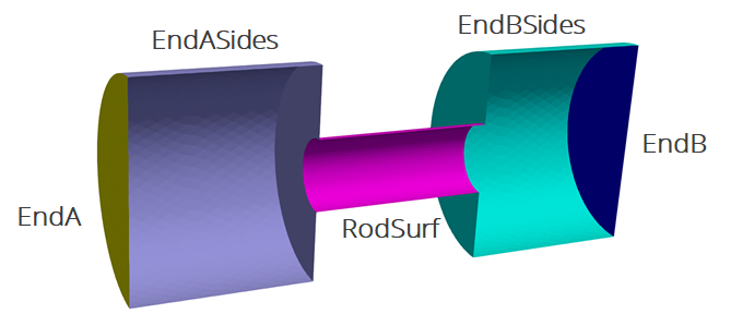
The problem also includes five separate named sidesets (EndA, EndB, EndASides, EndBSides, and RodSurf) applied on different surfaces of the mesh. Sidesets in aria are used to apply boundary conditions or do surface post-processing. Any surface not covered by a sideset will be treated as adiabatic, as will any sideset with no boundary condition applied to it.
The mesh file needed for this tutorial can be downloaded here, or it can be generated manually using the Cubit journal file below.
Cubit Journal File
undo on

create cylinder height 0.1 radius 0.01
create cylinder height 0.05 radius 0.03
create cylinder height 0.05 radius 0.03
volume 2 move z 0.05
volume 3 move z -0.05
subtract volume 1 from volume 2 3 keep
delete volume 2 3
merge all
imprint all
merge all

volume 1 size 0.003
volume 4 5 size 0.005

volume all tetmesh growth_factor 1.05
volume all scheme tetmesh
mesh volume all

block 1 add volume 1
block 1 name "CenterRod"
block 2 add volume 4
block 2 name "ClampA"
block 3 add volume 5
block 3 name "ClampB"


sideset 1 add surface 14
sideset 1 name "EndA"

sideset 2 add surface 18
sideset 2 name "EndB"

sideset 3 add surface 20
sideset 3 name "RodSurf"

sideset 4 add surface 13 12
sideset 4 name "EndASides"

sideset 5 add surface 17 19
sideset 5 name "EndBSides"

undo group begin
set exodus netcdf4 off
set large exodus file on
export mesh "mesh.g" overwrite
undo group end
5.1.1.3. Aria Input File
Every Aria simulation requires a text input file to define the problem. The following sections show how to set up that file to run a transient heat conduction problem using the geometry shown above.
Indentation is recommended but not required in an Aria input file. You can indent with tabs or spaces, or choose not to indent things at all - although we highly recommend using indentation (with spaces) to make a consistently readable input file and to avoid errors with commands going in the wrong scope.
Anything that starts with a # or a $ will be treated as a comment and ignored. Long lines can be split using \$, like this
# This is a comment
$ and so is this

# This is a single line command split on three lines
List of Blocks = block_1 block_2 block_3 \$
                 block_4 block_5 block_6 \$
                 block_7 block_8
5.1.1.3.1. Overall File Structure
The Aria input file is structured using nested blocks with Begin and End commands surrounding each block. The outermost block must always be the SIERRA block. Commands directly in this block are referred to as “Domain-level” commands. Other commands must go inside inner blocks, such as “Procedure” or “Aria Region”, and will be referred to as such. If you put a command in the wrong level, you will get an error when you try to run Aria.
Begin SIERRA Aria
  # Domain-level commands

  Begin Procedure AriaProcedure
    # Procedure-level commands

    Begin Solution Control Description
      # Solution control commands
    End

    Begin Aria Region myRegion
      # Region-level commands
    End
  End
End
5.1.1.3.2. Defining Materials
Scope: Domain
You must define a material to use for each block in your mesh. A material can be used on multiple blocks, but every block must have a material. The properties required for your material will depend on what equations you are solving. (For more information on material definition refer to Material Properties ).
A transient heat conduction problem like this requires four properties:
Density
Specific heat
Thermal Conductivity
A model for heat flux
The syntax for setting up a material block named “aluminum” with constant properties is shown below:
Begin Aria Material aluminum
    Density              = Constant value = 2770  # kg/m^3
    Specific Heat        = Constant value = 800.0 # J/kg-K
    Thermal Conductivity = Constant value = 175.0 # W/mK
    Heat Conduction      = Generalized
End   Aria Material aluminum
The general format for specifying a material property is:
PROPERTY = MODEL [MODEL ARGS]
Some common examples of different models are Constant, Polynomial, Scalar_String_Function, and many others. Each of these models requires a different set of arguments. Examples of how to use these are shown below.
Density              =  Constant               value = 100
Specific Heat        =  Polynomial             order=1 C0=1 C1=1 variable=density
Thermal conductivity =  User_Function          name = my_fcn X = time
Viscosity            =  Scalar_String_Function f = "2*temperature"
For a complete list of the available models to use for a given property, you can refer to the Material Properties section of the user manual. For example, to see all available models for density you could go to the density section.
5.1.1.3.3. Define the Finite Element Model
Scope: Domain
The finite element model section is where you indicate which mesh file to use and associate materials with the blocks and surfaces in the mesh.
Begin Finite Element Model FEModel
    Database Name = mesh.g
    Use Material aluminum for ClampA ClampB CenterRod
End   Finite Element Model FEModel
5.1.1.3.4. Linear Solver
Scope: Domain
Every problem requires at least one linear solver to use to solve the generated linear system. Aria includes several preset solvers that can be used for common problem types. For this example we will use the “Thermal_Symmetric” preset, which uses the CG solver with a Jacobi preconditioner.
Begin tpetra equation solver solve_temperature
  Begin Preset Solver
    Solver Type = Thermal_Symmetric
  End
End
5.1.1.3.5. Solution Control
Scope: Procedure
The solution control block defines how the Aria region gets executed - a single time for a steady-state problem or multiple times for a transient problem. When the problem is transient, this is also where you specify the time step selection method, time integration scheme, and other parameters related to time step selection.
$---------------------------------------------------
$       Define temporal solution parameters
$---------------------------------------------------
    Begin Solution Control Description
        Use System Main

        Begin System Main
            Begin Transient Solution_block_1
                Advance AriaRegion
            End
        End

$---------------------------------------------------
$           Specify time integration settings
$---------------------------------------------------
        Begin Parameters for Transient Solution_Block_1
            Start Time       = 0.0   # seconds
            Termination Time = 600.0 # seconds

            Begin Parameters for Aria Region AriaRegion
                Time Step Variation = Adaptive
                Initial Time Step Size = 0.05
                Time Integration Method = BDF2
                Maximum Time Step Size = 20.0
                Minimum Time Step Size = 0.01
                Predictor-Corrector Tolerance = 0.01
            End
        End
    End
5.1.1.3.6. Aria Region
Scope: Procedure
The Aria Region is where you specify nonlinear solution settings, what equation you are solving, boundary conditions, initial conditions, postprocessors, and output controls.
Before getting to the problem-specific selections, there are a few general settings required in the Region block:
Which linear solver to use
Nonlinear solution settings (strategy, tolerances, etc)
Which finite element model block (mesh) to use. Each region must be associated with exactly one mesh.
The following block shows a standard set of parameters, which we will use for this example.
Begin Aria Region AriaRegion

  $---------------------------------------------------
  $ Define linear and nonlinear solver parameters
  $---------------------------------------------------
  Use Linear Solver solve_temperature
  Nonlinear Solution Strategy  = Newton
  Maximum Nonlinear Iterations = 10
  Nonlinear Residual Tolerance = 1.e-6

  $-----------------------------------------------------------
  $ Specify which mesh model to use for this region
  $-----------------------------------------------------------
  Use Finite Element Model FEModel

  # other region commands
End
5.1.1.3.7. Governing Equation
Scope: Aria Region
The equations to solve are specified with one or more “EQ” lines. The important specifications on the EQ line are the equation name (Energy), the degree-of-freedom (DOF) name (Temperature), the location to solve the equation on (all_blocks), and the terms to activate in the equation (Mass and Diff).
#  NAME       DOF            LOCATION                 TERMS
EQ Energy for Temperature on all_blocks using Q1 with Mass Diff
This generates a governing equation of

The “mass” term is required for transient problems, and adds the  term, and the “diff” term adds the
  term.
term.
When we set up our material properies we defined that  when we set the heat conduction model as “Generalized”, so the overall governing equation we are solving is

5.1.1.3.8. Initial Conditions
Scope: Aria Region
Since this is a transient problem, initial conditions are required for all DOFs on all blocks. The syntax for setting initial conditions is very similar to the syntax used to set material properties
IC for DOF on BLOCK = MODEL [MODEL ARGS]
To set a constant initial condition for temperature of 300 K, we would use
IC for Temperature on all_blocks = constant value = 300 # K
To see what other models are available to use for initial conditions you can refer to the initial condition section in the user manual - common models include constant, user_function, and scalar_string_function.
5.1.1.3.9. Boundary Conditions
Scope: Aria Region
As with initial conditions and material properties, boundary conditions can be specified by selecting a model and providing its arguments in-line. There are two primary categories of boundary conditions in Aria - Dirichlet (which specify the DOF on the boundary) and Flux (which specify flux of the conserved quantity). The syntax for these is
BC Dirichlet for DOF on SIDESET = MODEL [MODEL ARGS]
BC Flux for EQUATION on SIDESET = MODEL [MODEL ARGS]
For this problem we are going to set Dirichlet (fixed temperature) boundary conditions on the ends of the clamps (EndA and EndB). To make the problem have some time variation, we will use a scalar string function to define a time-varying condition on one end of the domain.
BC Dirichlet for temperature on EndA = constant value = 300 # K
BC Dirichlet for temperature on EndB = scalar_string_function f = "350+100*sin(t/300)" # K
To see all the available boundary condition models, you can use the boundary condition section in the user manual.
5.1.1.3.10. Solution Output
Scope: Aria Region
To output our results, we need to define a Results Output block, which will define the name of the file we are writing to, which fields to write, and how often to write. For the example below, we will write the temperature solution field to a variable called “T” in heat_cond.e every 5 time steps. Output can also be specified at a given time interval instead of a step interval using At time 0 Increment = 0.1.
Begin Results Output AriaOutput
    Title Aria: Transient Training Model
    Database Name = heat_cond.e
    At Step 0 Interval = 5
    Nodal Variables = Solution->Temperature as T
End
5.1.1.4. Running Aria
Once you have finished setting up the input file, you are ready to run Aria. From a CEE unix environment, you can load the sierra module to access the latest release of Aria to run it on your local machine. To run it on 4 processors, you could use
$ module load sierra
$ launch -n 4 aria -i heat_cond_session1.i
5.1.1.4.1. Reading the Log File
As it runs, Aria will output continuously to a log file, by default with the same base name as your input file (e.g. “heat_cond_session1.log”). You can check the log file to monitor the job progress and to check that it is adequately solving your specified equations. The log file is also where you should look if the solution terminates with an error.
Transient solution_block_1: dt = 0.05
Transient Solution_Block_1, step 1, time 5.0000e-02, time step 5.0000e-02, 0.00% complete
Memory Usage: current = 302419968 (288.4 M), high-water-mark = 421240832 (401.7 M)
DEFAULTING PREDICTOR-CORRECTOR_BEGIN_AFTER_STEP = 3.

Equation System AriaRegion->main:
* Step  : Transient, Strategy: NEWTON, Time: 5.00e-02, Step: 5.00e-02
* Matrix: Solver: "solve_temperature", Unknowns: 6122, Nonzeros: 83476
* Mesh  : Processor 0 of 1: 30689 of 30689 elems, 6122 of 6122 nodes
  N O N L I N E A R                 L I N E A R
----------------------   --------------------------------------
Step  Resid    Delta     Itns  Status   Resid    Asm/Slv Time
---- -------- --------   ---- -------- -------- ---------------
  1 2.27e+03 5.80e+02     10       ok 4.07e-07 2.8e-02/2.6e-03
  2 9.25e-04 2.83e-04     14       ok 3.20e-07 2.8e-02/2.9e-03
  3 2.96e-10                     NoOp          2.7e-02
Termination reason: 2.95766e-10 < nonlinear_residual_tolerance(1e-06),
                and 0 < nonlinear_correction_tolerance(1e-06)
In the example log file output above, we can see that Aria took three nonlinear iterations to converge on the time step shown here, and that the final nonlinear residual was suitably low. The linear solver residuals and iteration counts are also shown here, and can be an indication of whether the solver you selected is struggling with the current problem (in this case it is not).
---------------------------------------------------
There were no errors encountered during parse
There was 1 warning encountered during parse
There were no errors encountered during execution
There were no warnings encountered during execution
+----+----+----+----+----+----+----+----+----+----+----+----+----+----+----+----
SIERRA execution successful.
    For region AriaRegion
      Number of timesteps            (failed) : 0
      Number of timesteps            ( total) : 190
      Number of nonlinear iterations ( total) : 394
    Memory Usage: current = 311021568 (296.6 M), high-water-mark = 421838848 (402.3 M)
At the end of the log file there is a summary showing that the problem executed successfully and the number of time steps, failed time steps, and nonlinear iterations.
If you want to output other quantities than just the temperature, you can also check the log file header (near the top) for a list of all available fields (nodal, face, element, and global) that are available to output.
Aria Region "Aria_region" has the following fields available for output:
  NODE_RANK Fields:
    * physical_coordinates
    * pp->HEAT_CONDUCTION
    * predicted_solution->TEMPERATURE
    * solution->TEMPERATURE
    * time_derivative_at_time->TEMPERATURE
  FACE_RANK Fields:
  * thermal_contact_status
  ELEMENT_RANK Fields:
    * current_element_volume
    * volume_change_ratio
  Global Variables:
    * p_inner
5.1.1.5. Viewing the Results
The two common tools used at Sandia for visualizing Exodus files are Ensight and Paraview. There are training courses available for both tools, so their use is not a focus of this tutorial. Examples shown here will use Paraview.
From a CEE unix environment with graphics, you can launch paraview using
$ module load viz
$ paraview heat_cond.e.4.0
Or if you have installed Paraview locally, you can launch it and select the exodus file from the appropriate file opening menu.
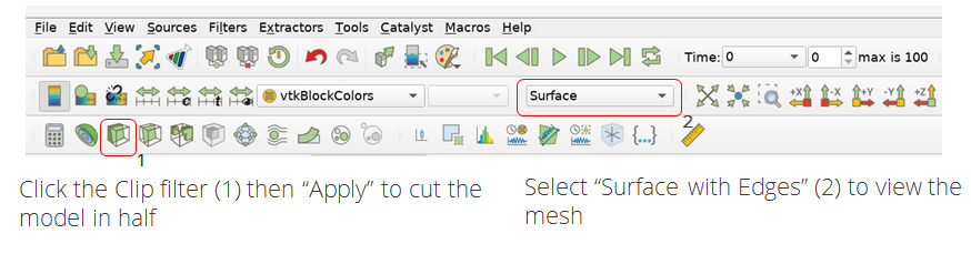
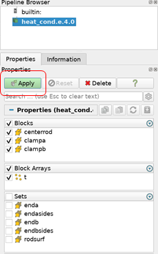
Once you have loaded it, you need to select which variables to show then click “Apply”
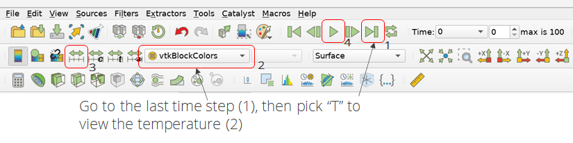
To show the temperature field on the object, you can
Go to the last time step
Select the temperature variable to show
If you showed temperature first the scale may be off. Rescale it.
Click the Play button to animate the results over time.
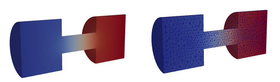
The result shows the temperature distribution is as-expected.
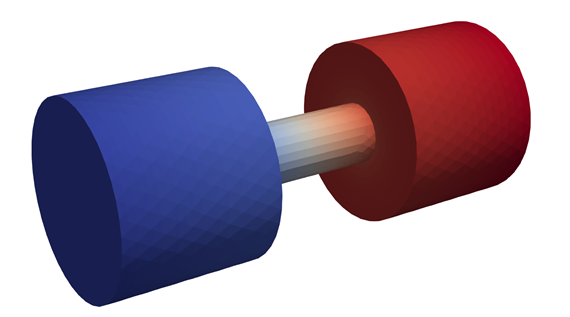
Next, we can slice the domain in half and look at the internal profile and the mesh details