5.1.5. Multiphysics Coupling
This tutorial builds on the prior Radiative Flux BCs tutorial and shows how couple multiple different types of equations (electrical and thermal transport). This module has also been recorded in prior trainings and is available here or in the player below.
5.1.5.1. Problem Files
The files required for this tutorial can be downloaded here, or found at $SIERRA100/TF/Aria (where SIERRA100=/projects/sierra100 in a CEE environment, or your Sierra test distribution otherwise).
5.1.5.2. Problem Domain/Mesh
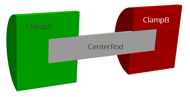
The geometry we will use for this tutorial is the same as the one used Basic Heat Conduction. It consists of three cylinders making a dumbbell shape, with three separate named blocks (ClampA, ClampB, and CenterRod). Blocks (volumetric sections in the mesh) are used in Aria to define different material properties, and can also be used to run post-processors on.
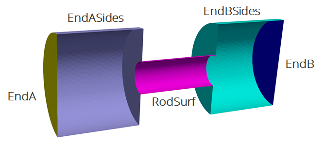
The problem also includes five separate named sidesets (EndA, EndB, EndASides, EndBSides, and RodSurf) applied on different surfaces of the mesh. Sidesets in aria are used to apply boundary conditions or do surface post-processing. Any surface not covered by a sideset will be treated as adiabatic, as will any sideset with no boundary condition applied to it.
The mesh file needed for this tutorial can be downloaded here, or it can be generated manually using the Cubit journal file shown in the Basic Heat Conduction tutorial.
5.1.5.3. Material Updates
Scope: Domain
To add an electrical transport equation, we need to define some additional material properties. These are the Electrical Conductivity and Current Density (the model for current flux). We must add these properties to both materials in order to solve for electrical transport on both of them.
Begin Aria Material aluminum
    Density              = Constant value = 2770  # kg/m^3
    Specific Heat        = Constant value = 800.0 # J/kg-K
    Thermal Conductivity = Constant value = 175.0 # W/mK
    Heat Conduction      = Generalized

    Electrical Conductivity = Constant Value = 10000 # S/m
    Current Density = Ohms_Law
End   Aria Material aluminum
Begin Aria Material ss304
    Density              = Constant value = 8000
    Specific Heat        = Polynomial Variable=Temperature order=1 C0=500 C1=0.1
    Thermal Conductivity = User_Function name=ssteel_k_function X=temperature
    Heat Conduction      = Generalized

    Electrical Conductivity = Constant Value = 0.1 # S/m
    Current Density = Ohms_Law
End   Aria Material ss304
5.1.5.4. Solver
Scope: Domain
For the prior examples we used a default thermal solver, but to more robustly solve this multi-physics problem we should use a different preset solver with a more robust preconditioner.
BEGIN TPETRA EQUATION SOLVER solve_temperature
  BEGIN PRESET SOLVER
    SOLVER TYPE = Multiphysics
  END
END TPETRA EQUATION SOLVER
5.1.5.5. Governing Equations
Scope: Aria Region
Next we will modify the EQ definitions to add a new current equation and add a source term to the energy equation for Joule heating. The source model (joule_heating) requires no additional arguments.
EQ Energy for Temperature on all_blocks using Q1 with Mass Diff Src
EQ Current for Voltage on all_blocks using Q1 with Diff

Source for Energy on all_blocks = joule_heating
This will solve  for voltage and add an energy source term of
  where
where  here is the electrical conductivity defined in the materials. These equations are now coupled in one direction since the energy equation depends on the voltage but the voltage solve is independent of temperature. If the electrical conductivity were defined as a function of temperature then it would introduce a two-way coupling between these equations and the current solve would change over time as the temperature changes. No changes to the input would be required to handle this two-way coupling, although the simulation may take more nonlinear iterations to reach convergence.
5.1.5.6. Boundary Conditions
Scope: Aria Region
The current equation has no mass term, so it does not require an initial condition. However, we must supply boundary conditions. For this problem we will set a constant voltage on one end of the domain and a constant current on the opposite end.
BC Dirichlet for Voltage on EndA = constant value = 0
BC Flux for Current on EndB = constant value = -100 # Amps/m2
5.1.5.7. Postprocessing
Scope: Aria Region
To see the current flux we can postprocess the current_density vector, and to see the energy source due to Joule heating we can postprocess the energy_source expression. By default energy_source is the sum of all source terms, but individual sources can be postprocessed using the Model keyword.
Postprocess value of expression energy_source on all_blocks as Esrc
Postprocess value of expression current_density on all_blocks as Current
5.1.5.8. Output
Scope: Aria Region
We now have several new fields to add to the results output block, including the new voltage value (solution->voltage) and the postprocessed values.
Begin Results Output AriaOutput
    Title Aria: Transient Training Model
    Database Name = heat_cond.e
    At Step 0 Interval = 5
    Nodal Variables = Solution->Temperature as T
    Nodal Variables = Solution->Voltage as V
    Nodal Variables = Current
    Nodal Variables = HeatFlux
    Nodal Variables = ConvFlux
    Nodal Variables = RadFlux
    Nodal Variables = Esrc

    Global Variables = FluxA
    Global Variables = FluxB
    Global Variables = ClampConvLoss
    Global Variables = RodConvLoss
End
5.1.5.9. Running Aria
Once you have finished setting up the input file, you are ready to run Aria. From a CEE unix environment, you can load the sierra module to access the latest release of Aria to run it on your local machine. To run it on 4 processors, you could use
$ module load sierra
$ launch -n 4 aria -i heat_cond_session5.i
5.1.5.10. Viewing the Results
From a CEE unix environment with graphics, you can launch paraview using
$ module load viz
$ paraview heat_cond.e.4.0
Or if you have installed Paraview locally, you can launch it and select the exodus file from the appropriate file opening menu.
Once you have loaded it, you need to select which variables to show then click “Apply”.
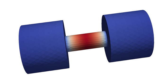
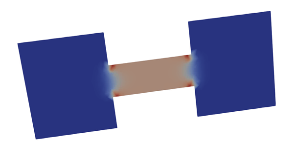
To show the temperature on the center rod, you can
Go to the last time step
Select the “T” variable to show
Rescale the color scale if needed
The temperature is highest in the center rod, where the electrical conductivity is lowest.
To view the energy source, you can
Slice the domain and click “Apply”
Select the “Esrc” variable
As expected, the energy source is concentrated in the low conductivity center rod.
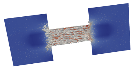
To visualize the current flux, you can
Select the “Glyph” filter
Apply a scaling of 1e-5
Click “Apply”
The current is highest through the narrow section of the domain, as expected.