5.1.6. Advanced Postprocessing
This tutorial builds on the prior Multiphysics Coupling tutorial and shows how to do more advanced postprocessing, extracting values at specific points and evaluating custom functions. This module has also been recorded in prior trainings and is available here or in the player below.
5.1.6.1. Problem Files
The files required for this tutorial can be downloaded here, or found at $SIERRA100/TF/Aria (where SIERRA100=/projects/sierra100 in a CEE environment, or your Sierra test distribution otherwise).
5.1.6.2. Problem Domain/Mesh
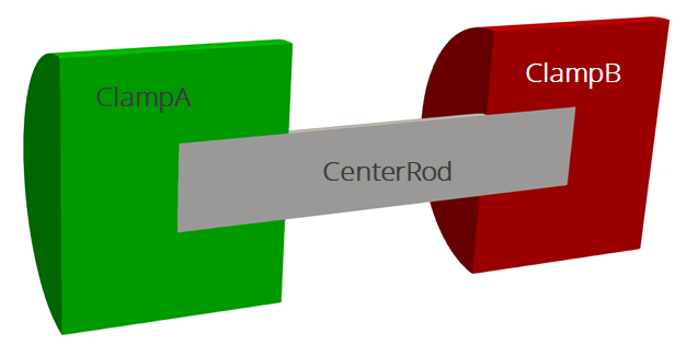
The geometry we will use for this tutorial is the same as the one used Basic Heat Conduction. It consists of three cylinders making a dumbbell shape, with three separate named blocks (ClampA, ClampB, and CenterRod). Blocks (volumetric sections in the mesh) are used in Aria to define different material properties, and can also be used to run post-processors on.
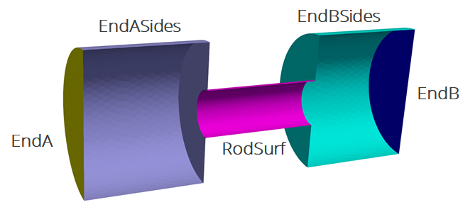
The problem also includes five separate named sidesets (EndA, EndB, EndASides, EndBSides, and RodSurf) applied on different surfaces of the mesh. Sidesets in aria are used to apply boundary conditions or do surface post-processing. Any surface not covered by a sideset will be treated as adiabatic, as will any sideset with no boundary condition applied to it.
The mesh file needed for this tutorial can be downloaded here, or it can be generated manually using the Cubit journal file shown in the Basic Heat Conduction tutorial.
5.1.6.3. Extract Value at a Point
Scope: Aria Region
The first post-processor we will add is to extract a variable at a specific location in the mesh (0,0,0).
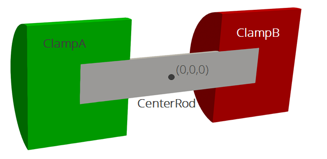
To extract the value or an expression (solution DOF or any material property) at a given point, we can use a data probe.
Postprocess value of expression temperature at point 0 0 0 as Trod
5.1.6.4. Custom Functions
Scope: Aria Region
We can also use string functions to post-process any arbitrary quantity we might be interested in for our analysis. For example, if we wanted to calculate the average temperature in Celsius on the center rod and output a field with the ratio of voltage to internal energy, we could define these two post-processors.
Postprocess average of function "temperature-273.15" on CenterRod as TavgC
Postprocess value of function "voltage / (density*specific_heat*temperature)" on all_blocks as VEratio
5.1.6.5. Heartbeat Output
Scope: Aria Region
In the prior examples we have output all our data to an Exodus file in the Results Output block. However, it is common to output global variables to a text file at a higher frequency.
Begin Heartbeat AriaTxtOutput
    Stream name = stats.csv
    Format = csv
    At Step 0 increment = 1
    Variable is Global time
    Variable is Global FluxA
    Variable is Global FluxB
    Variable is Global ClampConvLoss
    Variable is Global RodConvLoss
    Variable is Global Trod
    Variable is Global TavgC
End
5.1.6.6. Results Output
Scope: Aria Region
We created a new nodal field (VEratio) with the custom post-processor. To be able to view it, we need to add it to the results output block.
Begin Results Output AriaOutput
    Database Name = heat_cond.e
    At Step 0 Interval = 5
    Title Aria: Transient Training Model
    Nodal Variables = Solution->Temperature as T
    Nodal Variables = Solution->Voltage as V
    Nodal Variables = Current
    Nodal Variables = HeatFlux
    Nodal Variables = ConvFlux
    Nodal Variables = RadFlux
    Nodal Variables = Esrc
    Nodal Variables = VEratio

    Global Variables = FluxA
    Global Variables = FluxB
    Global Variables = ClampConvLoss
    Global Variables = RodConvLoss
End
5.1.6.7. Running Aria
Once you have finished setting up the input file, you are ready to run Aria. From a CEE unix environment, you can load the sierra module to access the latest release of Aria to run it on your local machine. To run it on 4 processors, you could use
$ module load sierra
$ launch -n 4 aria -i heat_cond_session6.i
5.1.6.8. Viewing the Results
From a CEE unix environment with graphics, you can launch paraview using
$ module load viz
$ paraview heat_cond.e.4.0
Or if you have installed Paraview locally, you can launch it and select the exodus file from the appropriate file opening menu.
Once you have loaded it, you need to select which variables to show then click “Apply”.
To show the post-processed field (VEratio), you can
Go to the last time step
Select the “VEratio” variable to show
Rescale the color scale if needed
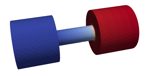
The result shows the custom calculated quantity.
Note
You can use a calculator filter in Paraview to do custom calculations as well, but you only have access to quantities you already output. In this example, we did not output specific_heat or density, so we would not be able to calculate VERatio in Paraview. It is possible to use Aria to postprocess additional quantities based on the already computed results. The next section demonstrates that process to add specific_heat and density to the results file.
5.1.6.9. Postprocessing Additional Quantities
As an example of doing additional postprocessing based on existing results we will add specific_heat and density to a new results file for this case.
The input file needed to do this is available from:
The process starts by copying the initial input file and making the following modifications:
Add a new finite element model referencing the results of the prior run:
Begin Finite Element Model FEModel
    Database Name = mesh.g

    Use Material aluminum for ClampA ClampB
    Use Material ss304 for CenterRod

End   Finite Element Model FEModel

Begin Finite Element Model ExistingResults
    Database Name = heat_cond.e
End   Finite Element Model
Add an input output region to read the data, transfers to send that data to the Aria region that will do the additional postprocessing, and update the time step settings to let the input output region control the time step. Note that since the meshes are identical, one can use Include All Blocks in these transfers rather than have to list each block pairing:
Begin Solution Control Description
    Use System Main

    Begin Initialize init
        Advance IORegion
        advance AriaRegion
        transfer existing_to_aria_init
    End

    Begin System Main
        Use Initialize init
        Begin Transient solution_block_1
            Advance IORegion
            Transfer existing_to_aria
            Advance AriaRegion
        End   Transient solution_block_1
    End   System Main

    Begin Parameters for Transient Solution_Block_1
        Start Time       = 0.0        # seconds
        Termination Time = {end_time} # seconds

        Begin Parameters for Aria Region AriaRegion
            Time Step Variation = FIXED
            Initial Time Step Size = {end_time}
            Time Integration Method = BDF2
        End   Parameters for Aria Region AriaRegion

    End   Parameters for Transient Solution_Block_1
End

Begin Input_Output Region IORegion
    Use Finite Element Model ExistingResults
    TIMESTEP ADJUSTMENT INTERVAL = 1
End

Begin Transfer existing_to_aria_init
    Copy Volume Nodes From IORegion to AriaRegion

    Begin Send Blocks
        Include All Blocks
    End
    Begin Receive Blocks
        Include All Blocks
    End

    # Otherwise one can also specify a subset of blocks to transfer
    # Send Block CenterRod to CenterRod
    # Send Block ClampA to ClampA
    # Send Block ClampB to ClampB

    Send field T state none To solution->temperature state new
    Send field V state none To solution->voltage state new
    Send field T state none To solution->temperature state old
    Send field V state none To solution->voltage state old
End

Begin Transfer existing_to_aria
    Copy Volume Nodes From IORegion to AriaRegion

    Begin Send Blocks
        Include All Blocks
    End
    Begin Receive Blocks
        Include All Blocks
    End

    Send field T state none To solution->temperature state new
    Send field V state none To solution->voltage state new
End
Switch the Aria equation definitions to XFER and disable the boundary conditions:
EQ Energy for Temperature on all_blocks using Q1 with XFER #Mass Diff Src
EQ Current for Voltage on all_blocks using Q1 with XFER #Diff

IC for Temperature on all_blocks = constant value = 300 # K

#Source for Energy on all_blocks = joule_heating

#BC Dirichlet for temperature on EndA = constant value = 300 # K
#BC Dirichlet for temperature on EndB = constant value = 300 # K

Mesh Group clamp_conv = EndASides EndBSides
Mesh Group rad_surfs = all_surfaces - EndA - EndB

#BC Flux for Energy on clamp_conv = Nat_Conv H=5 T_ref=250
#BC Flux for Energy on RodSurf = Nat_Conv H=10 T_ref=250

#BC Flux for Energy on rad_surfs = Rad T_ref = 250 Crad = {e*sigma}

#BC Dirichlet for Voltage on EndA = constant value = 0
#BC Flux for Current on EndB = constant value = -100 # Amps/m2
Add the additional desired postprocessors and include them in the results output:
Postprocess value of expression specific_heat on all_blocks as Cp
Postprocess value of expression density on all_blocks as rho

...

Begin Results Output AriaOutput

    ...

    Nodal Variables = Cp
    Nodal Variables = rho

    ...
End