5.1.1. Laminar Flow Over A Cylinder
This tutorial shows how to set up a flow over cylinder in Fuego. This module has also been recorded in prior trainings and is available here or in the player below.
5.1.1.1. Problem Files
The files required for this tutorial can be downloaded here, or found in a CEE environment at /projects/sierra100/TF/Fuego.
5.1.1.2. Problem Domain/Mesh
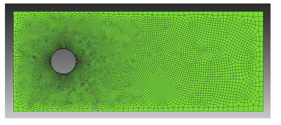
In this tutorial we will be simulating a 2D laminar flow over a cylinder cross-section, where the mesh is shown below
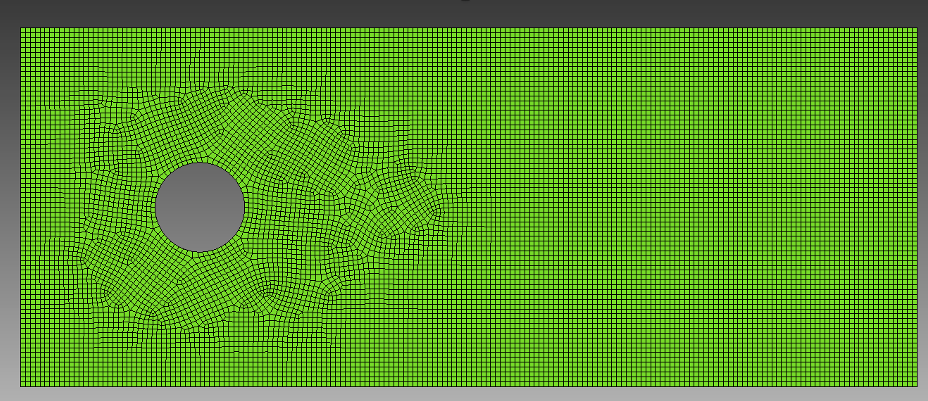
The mesh file needed for this tutorial can be downloaded here, or it can be generated manually using the Cubit journal file below.
Cubit Journal File
undo on
# { D = 0.1 }

brick x {10*D} y {4*D} z 1
create cylinder height 1 radius {D/2}
move volume 2 x {-3*D}
subtract volume 2 from volume 1

block 1 add surface 11
block all element type QUAD4
surface 11 size {0.054*D}
mesh surface 11

sideset 1 add curve 3
sideset 2 add curve 1
sideset 3 add curve 2 4
sideset 4 add curve 16
set large exodus file on
export genesis "cyl_base.g" dimension 2 block all overwrite
5.1.1.3. Fuego Input File
Every Fuego simulation requires a text input file to define the problem. The following sections show how to set up that file to run a the laminar flow problem using the geometry shown above.
Indentation is recommended but not required in an Fuego input file. You can indent with tabs or spaces, or choose not to indent things at all - although we highly recommend using indentation (with spaces) to make a consistently readable input file and to avoid errors with commands going in the wrong scope.
Anything that starts with a # or a $ will be treated as a comment and ignored. Long lines can be split using \$, like this
# This is a comment
$ and so is this

# This is a single line command split on three lines
List of Blocks = block_1 block_2 block_3 \$
                 block_4 block_5 block_6 \$
                 block_7 block_8
5.1.1.3.1. Overall File Structure
The Fuego input file is structured using nested blocks with Begin and End commands surrounding each block. The outermost block must always be the SIERRA block.
Commands directly in this block are referred to as “Domain-level” commands. Other commands must go inside inner blocks, such as “Procedure” or “Fuego Region”, and will be referred
to as such. If you put a command in the wrong level, you will get an error when you try to run Fuego.
Begin SIERRA Fuego
  # Domain-level commands

  Begin Procedure FuegoProcedure
    # Procedure-level commands

    Begin Solution Control Description
      # Solution control commands
    End

    Begin Fuego Region myRegion
      # Region-level commands
    End
  End
End
For more information on the Fuego input file, please see Anatomy of an Input Deck.
5.1.1.3.2. Defining Materials
Scope: Domain
You must define a material to use for each block in your mesh. A material can be used on multiple blocks, but every block must have a material. The properties required for your material will depend on what equations you are solving.
Generally in Fuego only one material is usually defined. In this particular example for a laminar flow over a cylinder, we need to specify both a density and (dynamic) viscosity for the material
Begin Property Specification for Fuego Material air
  Density   = 1.2 #kg/m3
  Viscosity = 1.8e-5 #Pa s
End   Property Specification for Fuego Material air
In this material definition, we have defined both the density and viscosity as constants.
In general, these properties will be in the units of your problem setup, which we will define in Fuego Region Parameters). We will use MKS (meters, kilograms, and seconds) as our length, mass, and time scales, respectively, for this problem.
5.1.1.3.3. Define The Finite Element Model
Scope: Domain
The finite element model model defines the mesh file that is used in the simulation, the database type (usually ExodusII), and the parallel decomposition method (RIB or RCB). Additionally, the finite element model is used to associate mesh blocks with the materials we defined in the previous Defining Materials
Begin Finite Element Model cylMesh
    Database Name = cyl_base.g
    Database Type = ExodusII
    Decomposition Method = RIB

    # ASSIGN MATERIALS TO BLOCKS
    Begin Parameters for Block block_1
      Material air
    End   Parameters for Block block_1

End   Finite Element Model cylMesh
Typically in Fuego you do not need a large amount of blocks, except in a few cases:
Elements of different topologies (hex, tet, wedge, pyramid) must go in separate blocks
You may want different initial conditions in some places based on block specifications
5.1.1.3.4. Time Stepping Control
Scope: Procedure
Next we must set up some of the rules and parameters for how we want to set up time stepping for this transient problem.
Begin Fuego Procedure Fuego_procedure

    Time Start = 0.0, Stop = 10.0, Status Interval = 10

    begin time control
        BEGIN TIME STEPPING BLOCK  time_block
            START TIME IS   0.0
            TIME STEP = 1e-3
            BEGIN PARAMETERS FOR FUEGO REGION fuego_region
                TRANSIENT STEP TYPE IS automatic
                CFL LIMIT = 5.0
                TIME STEP CHANGE FACTOR = 1.5
            END   PARAMETERS FOR FUEGO REGION fuego_region
        END   TIME STEPPING BLOCK time_block

        Termination time = 1e6
    end time control
Typically in this block we set the start and end times. The status interval is used to print more diagnostics at the specified interval (every 10 steps in this case).
In the time stepping control we specify the initial timestep  , and to also automatically adapt the time step based on the global CFL limit defined as

where  is the element velocity,
  is the timestep, and
  is an element length scale. This CFL condition is computed inside each element and the global
timestep is chosen based on the global maximum computed CFL on all of the elements in your simulation.
is an element length scale. This CFL condition is computed inside each element and the global
timestep is chosen based on the global maximum computed CFL on all of the elements in your simulation.
Most Fuego problems are transient, but steady problems can be solved using a pseudo-transient approach.
5.1.1.3.5. Fuego Region Parameters
Scope: Region
Here we will set up some parameters in the Fuego region
Begin Fuego Region Fuego_region

    # SET THE UNITS
    Set unit system to MKS

    # DECLARE WHICH MESH/FINITE ELEMENT MODEL TO USE
    Use Finite Element Model cylMesh
Here we tell the region which finite element model to use (the one defined in Define The Finite Element Model) and unit system to use MKS (default to CGS if not specified).
One can define their own custom length/mass/time scales using the following commands in the Fuego region scope:
# Does the same thing as “SET UNIT SYSTEM TO MKS”
SET LENGTH UNIT CONVERSION FACTOR = 100.0
SET MASS   UNIT CONVERSION FACTOR = 1000.0
SET TIME   UNIT CONVERSION FACTOR = 1.0
SET TEMPERATURE UNITS = KELVIN
# use a non-standard mm-g-s unit system
SET LENGTH UNIT CONVERSION FACTOR = 0.1
SET MASS   UNIT CONVERSION FACTOR = 1.0
SET TIME   UNIT CONVERSION FACTOR = 1.0
For more information on setting length/mass/time scales see Units.
5.1.1.3.6. Solution Options
Scope: Region
The solution options block defines what equations to solve, and sets various numerical algorithm choices
Begin Solution Options
    Coordinate System = 2D
    Projection Method = Fourth_Order Smoothing with Timestep Scaling

    # DEFINE WHAT EQUATIONS TO SOLVE
    Activate Equation Continuity
    Activate Equation X_Momentum
    Activate Equation Y_Momentum

    # DEFINE NONLINEAR ITERATION SETTINGS
    Minimum Number of Nonlinear Iterations = 1
    Maximum Number of Nonlinear Iterations = 2

    # DEFINE ADVECTION SCHEME
    Upwind Method is MUSCL
    UPWIND LIMITER IS SuperBee

End   Solution Options
We will go into detail on a few sub-blocks of this input file snippet:
Projection Method = Fourth_Order Smoothing with Timestep Scaling
The common choice here for the pressure projection is the fourth order smoothing with timestep scaling. There are more advanced options shown in Smoothing Method, but for most problems this will suffice.
# DEFINE WHAT EQUATIONS TO SOLVE
Activate Equation Continuity
Activate Equation X_Momentum
Activate Equation Y_Momentum
This defines which equations you want Fuego to solve. In this case, since we are running a two-dimensional problem, we want to activate the continuity equation, as well as the x (streamwise) and y (wall normal) momentum equations (see Equations To Solve for more on what equations you can activate). For more detail on the continuity and momentum equations Fuego solves, please see Low Mach Number Equations.
# DEFINE NONLINEAR ITERATION SETTINGS
Minimum Number of Nonlinear Iterations = 1
Maximum Number of Nonlinear Iterations = 2
This sets the minimum and maximum number of nonlinear iterations for Fuego to take when solving the above equations. The default nonlinear residual tolerance is  , which is small enough
where Fuego will always take the maximum number of nonlinear iterations. For more advanced control, you can set a target nonlinear tolerance per equation (see Nonlinear Iteration Settings).
, which is small enough
where Fuego will always take the maximum number of nonlinear iterations. For more advanced control, you can set a target nonlinear tolerance per equation (see Nonlinear Iteration Settings).
# DEFINE ADVECTION SCHEME
Upwind Method is MUSCL
UPWIND LIMITER IS SuperBee
We must choose which algorithm to use to handle the advection term (“Upwind Method”) in the transport equations. Two common upwinding methods are UPW and MUSCL. UPW is a fully upwinded advective stabilization, which is more dissipative but is low order (1st order). MUSCL is a higher order and less dissipative advection scheme and is 2nd order accurate, but general needs an upwind limiter. For a more advanced discussion on the topic, see Advection Methods.
5.1.1.3.7. Boundary Conditions
Scope: Region
Boundary conditions are set in the following input file commands:
Begin Inflow Boundary Condition on Surface surface_1
    X_Velocity = (2000*1.8e-5)/(1.2*0.1)
    Y_Velocity = 0.0
End

Begin Open Boundary Condition on Surface surface_2
    Pressure = 0.0
End

Begin Symmetry Boundary Condition on Surface surface_3
End

Begin Wall Boundary Condition on Surface surface_4
    post process yplus
End
For reference, the mesh with labeled surfaces is shown below
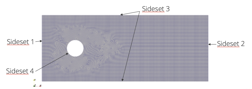
In this mesh we have included the four sidesets that were defined. Sideset 1, 2 and 3 represent the free flow boundaries and sideset 4 represents the solid wall cylinder boundary.
A constant inflow velocity is set on surface_1 in the x (streamwise) direction. This corresponds to a uniform inflow. An outflow boundary condition is set on surface_2, where the pressure
is specified. On Surface 3, we specify a symmetry boundary condition which effectively allows the flow to “slip” on those surfaces, and do not take parameters in the symmetry boundary condition
input block. Last, we specify a wall boundary condition on surface_4, which is effectively a no-slip condition. In this wall boundary condition block, we ask to postprocess “yplus” ( ), see
Wall Functions; Momentum for its definition.
), see
Wall Functions; Momentum for its definition.
5.1.1.3.8. Results Output
Scope: Region
Results are typically read into an Exodus file, at regular intervals set by the user.
Begin Results Output Label Fuego_output
    Database Name = results/cylinder.e
    At Time 0, Interval = 0.1
    Title Turbulent backward facing step flow
    Nodal Variables = Pressure as P
    Nodal Variables = X_Velocity as Ux
    Nodal Variables = Y_Velocity as Uy
    Nodal Variables = yplus
End
Here, we set the name of the file into the results/ directory. If this directory does not already exist, then it will be created. We also wish to output various nodal fields pertaining
to the solution of this problem, including pressure, velocity, and the yplus values we calculated in the previous section. By putting “x” and “y” suffix allows for visualization applications like Paraview
and Ensight to store them in a vector field for easier visualization. For reference, the logfile will display all fields (global, element, and nodal) available for output shown below:
Fuego Region "Fuego_region" has the following fields available for output:
  GLOBAL Variables:
    * AREA_X_surface_1
    * mass_flow_rate_surface_2
    * surface_4_MAXIMUM_YPLUS
  NODE_RANK Fields:
    * pressure
    * x_velocity
    * y_velocity
    * yplus
  ELEMENT_RANK Fields:
    * CFL
    * ap_ip
    * mass_flux
Any of the fields listed here can be output into an exodus file.
5.1.1.4. Running Fuego and Reading The Logfile
To run Fuego, open a terminal and navigate to where your input files and mesh files are located, and run the following commands:
module load sierra
mpirun -n 4 fuego -i flow_over_cylinder.i -o logfile.log
The first command loads the sierra module which is available on most brokered workstations. If these modules do not exist for your specific workflow, please contact your IT team for information
on how to load the sierra/Fuego environment on your particular machine. The second command will launch a parallel job with 4 processors running the fuego executable. The -i option is used
to specify the input file you want to run Fuego with, and the -o option will specify the logfile output name. This is an optional command, and omitting it will default to naming the logfile as
flow_over_cylinder.log.
Some things to look for in a logfile involve
Error messages (if something went wrong)
Warnings (deprecation warnings, assumed defaults)
Solution progression
Appropriately small non-linear residual values
Linear solver performance
Maximum DOF values
Time step info
We will make some general observations in this snippet from the logfile.
Step 2    , Time = 3.750e-03, dT = 2.250000e-03, Simulation is   0.0% complete

Fuego      Nonlinear Residuals of the Equation Sets     Linear    Linear
Nonlinear      Cell Reynolds number(max) =     250.7      Solver    Solver
Iteration              CFL(max) =    0.1658             Iterations Residual   DOF Min    DOF Max
--------- --------------------------------------------- ---------- --------  ---------- ----------
1 of  2 : SubMechanicsManager
1 of  1 :   MomentumSubMech
              X_Momentum                   = 7.06e-03      2      2.42e-12   0.00e+00   1.51e+00
              Y_Momentum                   = 7.40e-04      2      5.02e-12  -6.93e-01   6.80e-01
              Continuity                   = 1.45e-04      16     2.83e-09  -9.17e-01   2.33e+00
                Velocity pre-correction ----------------------------------->     0.00       1.51
                Velocity post-correction ---------------------------------->     0.01       0.68
Fuego      Nonlinear Residuals of the Equation Sets     Linear    Linear
Nonlinear      Cell Reynolds number(max) =     250.7      Solver    Solver
Iteration              CFL(max) =    0.2487             Iterations Residual   DOF Min    DOF Max
--------- --------------------------------------------- ---------- --------  ---------- ----------
2 of  2 : SubMechanicsManager
1 of  1 :   MomentumSubMech
              X_Momentum                   = 4.78e-05      2      3.15e-12   0.00e+00   6.85e-01
              Y_Momentum                   = 1.67e-05      2      4.76e-12  -3.08e-01   3.25e-01
              Continuity                   = 4.98e-05      13     3.24e-09  -3.86e-01   5.83e-01
                Velocity pre-correction ----------------------------------->     0.00       0.69
                Velocity post-correction ---------------------------------->     0.02       0.62
This is a typical output in the logfile you will see when running Fuego. Here we show the maximum CFL number, as well as the performance of the equations systems and their linear solver residuals. You’ll want to make sure that your nonlinear residual is going down, and that for each nonlinear residual step that the linear solver residual is suitably small (O(1e-10)) to ensure nonlinear convergence of the solution. Also the DOF (degrees of freedom) max and min for each equation system is also shown. If these are unnecessary high (or low), there might be some issue you need to address. Be sure to read the logfile during execution to catch any problems, and make sure that the logfile is outputting what you expect it to.
5.1.1.5. Viewing Results
From a CEE unix environment with graphics, you can launch paraview using
module load viz
paraview cylinder.e.4.0
Or if you have a local paraview installation, use that and open the exodus file appropriately.
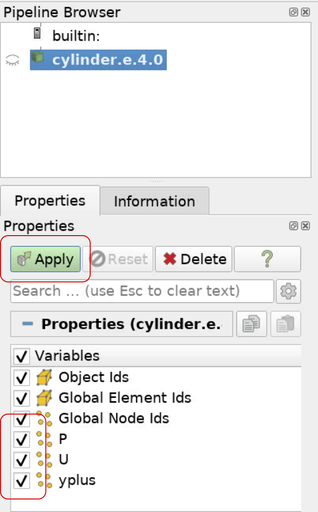
Once you have loaded paraview, you need to select which variables to show and click “Apply”
Once the variables are loaded, you can visualize the flow field using paraview
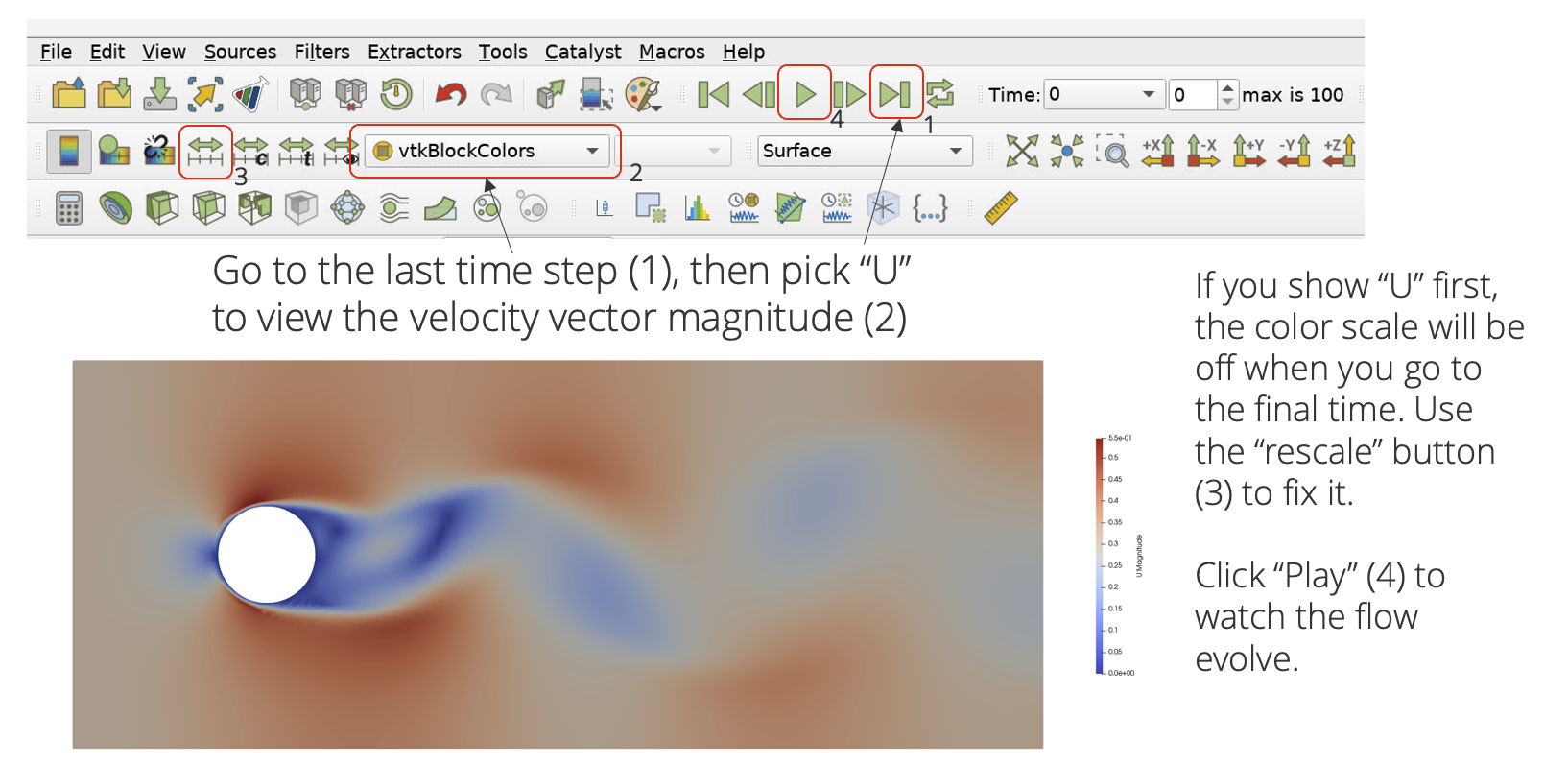
Here we color the mesh using the velocity field. In the case of a vector field, this is visualized as the vector magnitude. Notice the vortex shedding pattern.
We can visualize this vortex shedding pattern a little differently by coloring the solution with the y-component of the velocity field
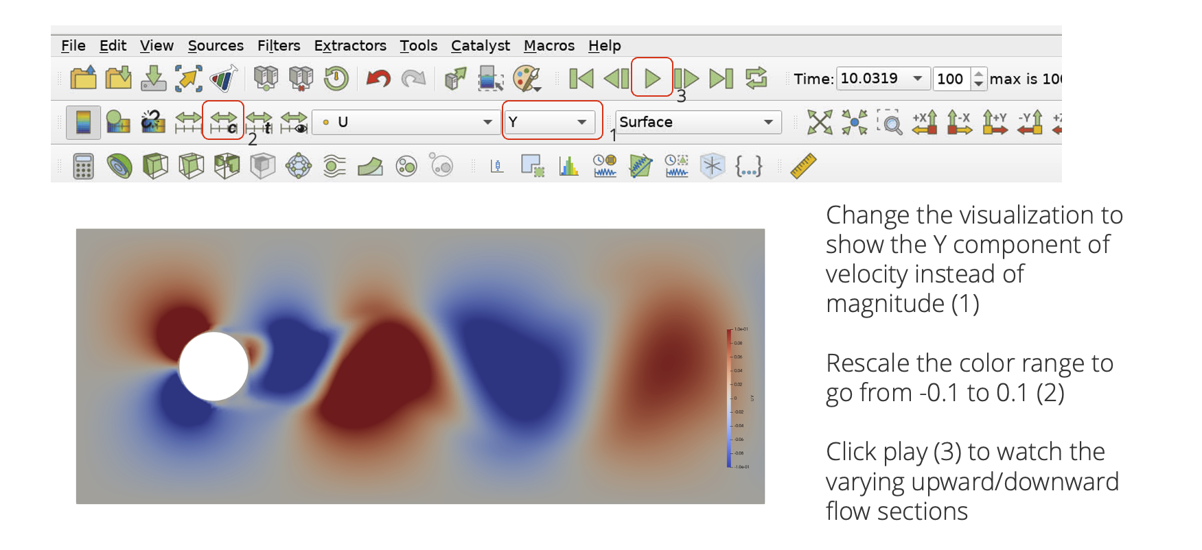
Hit the play button and observe the vortex shedding pattern. At what time does the vortex shedding begin? Is it periodic? Feel free to play around with visualizing different fields.
5.1.1.6. Changing the Mesh
Let us use a more refined mesh at the cylinder walls. Open the cyl_better.jou file and copy/paste into Cubit, or alternatively run it in command line mode
module load sierra
cubit -nographics -batch cyl_better.jou
Running the journal file will make a new mesh named cyl_better.g. Let’s change the mesh file in the finite element block and re-run the simulation.
Begin Finite Element Model cylMesh
    Database Name = cyl_better.g
    #other stuff
End Finite Element Model cylMesh
module load sierra
mpirun -n 4 fuego -i flow_over_cylinder.i
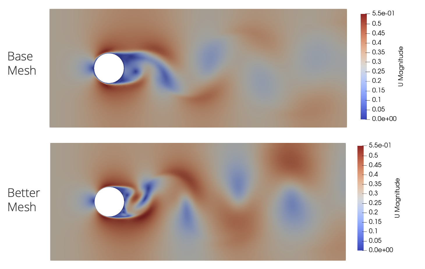
Let’s take a look at the new results, colored by the velocity vector magnitude, compared to the old mesh
Notice in the execution, while the element count between the two meshes were close, this new mesh took more time steps. This is due to the CFL condition we have placed on the problem
Where the elements near the cylinder wall are now smaller than the previous mesh. Therefore, all things being otherwise equal, the time step must shrink to accommodate this.
Compared to the old and new mesh, we see much better resolution of the vortex shedding event, especially near the cylinder.
5.1.1.7. Troubleshooting
In general, if your simulation fails to run correctly, or produces results different from what you expected, here are some steps you can take:
Check if SAW highlighted any syntax in your input file
Check the log file! Look for:
The words “Error” and “Warning”
High max CFL
Linear and nonlinear residual non-convergence
High maximum velocities, or large velocity corrections
Visualize the solution (ParaView), and look for anomalous regions of flow