5.1.4. Conjugate Heat Transfer

This tutorial shows how to set up a conjugate heat transfer (CHT) problem. This module has also been recorded in prior trainings and is available here or in the player below.

For problems with solid heat conduction and non-isothermal flow, you can use the combined fuego_aria` executable to run a conjugate heat transfer simulation. A description of the proposed problem is shown below

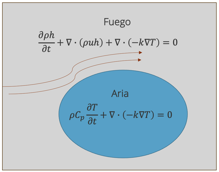
Here, a heat transfer equation is solved in Aria inside the cylinder domain, and an enthalpy transport equation will be solved in the Fuego (exterior) domain. The coupling between the cylinder temperature computed in Aria and the enthalpy in Fuego at the wall will be done through an iterative procedure illustrated below

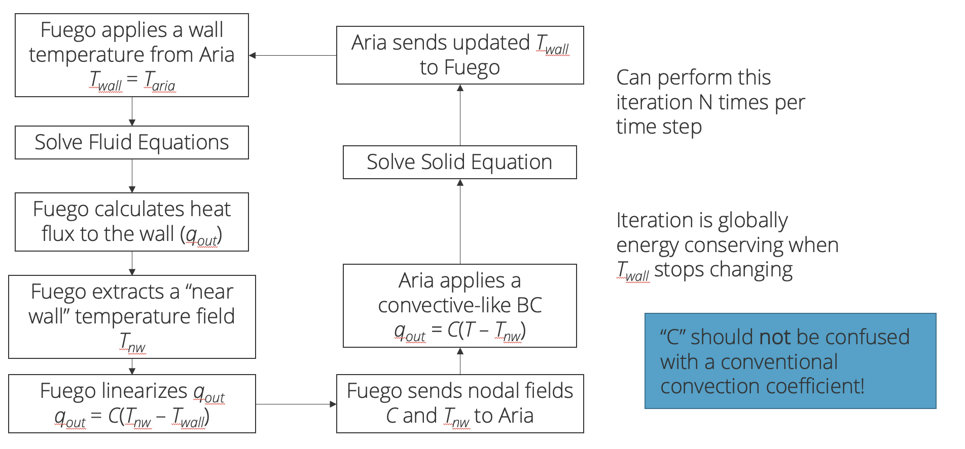
In this particular coupling procedure, Aria will send a wall temperature to Fuego, and Fuego, after doing a fluid solve, will send back a heat flux back to Aria. This is a conditionally stable procedure and in general will be 2nd order accurate.

5.1.4.1. Problem Files

The files required for this tutorial can be downloaded here, or found in a CEE environment at /projects/sierra100/TF/Fuego.

Fuego input file

Cylinder mesh file

Pipe mesh file

Training slides

5.1.4.2. Problem Domain/Mesh

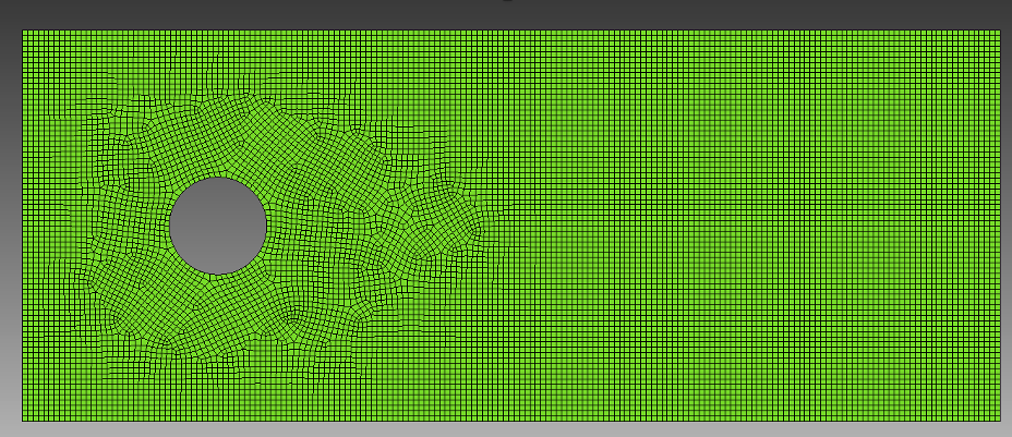
In this tutorial we will be simulating a 2D CHT problem over a cylinder cross-section, where the Fuego mesh (cyl_base.g) is shown above and the Aria mesh (pipe.g) is shown below

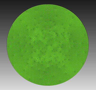
In the previous tutorials, we did not need to mesh the interior of the cylinder. However, since we are now solving a heat transfer problem inside the cylinder using Aria, we need to mesh the cylinder.

The mesh files needed for this tutorial can be downloaded in the links provided above, or it can be generated manually using the Cubit journal file below.

Cubit Journal File

undo on
# { D = 0.1 }

brick x {10*D} y {4*D} z 1
create cylinder height 1 radius {D/2}
move volume 2 x {-3*D}
subtract volume 2 from volume 1

block 1 add surface 11
block all element type QUAD4
surface 11 size {0.054*D}
mesh surface 11

sideset 1 add curve 3
sideset 2 add curve 1
sideset 3 add curve 2 4
sideset 4 add curve 16
set large exodus file on
export genesis "cyl_base.g" dimension 2 block all overwrite

reset

create cylinder height 1 radius {D/2}
move volume 1 x {-3*D}
block 1 add surface 3
block all element type QUAD4
surface 3 size {0.01*D}
mesh surface 3

sideset 1 add curve 2
set large exodus file on
export genesis "pipe.g" dimension 2 block all overwrite

5.1.4.3. Fuego Aria Input File

There are three things we will cover in this section

Activating an enthalpy equation in Fuego for non-isothermal flow
Adding in an Aria region and Aria materials
Defining the coupling and transfers between Fuego and Aria

The input file we are using can be found here.

5.1.4.3.1. Activating Enthalpy

For non-isothermal flow, we need enthalpy, specific heat, thermal conductivity, and a reference temperature

Scope: Domain

Begin Property Specification for Fuego Material air
   Density   = 1.2
   Viscosity = 1.8e-5
   Thermal_conductivity  = 0.025
   Specific_heat         = 1000
   Function For Enthalpy = Hfunc
   Reference Temperature = 300.0
End   Property Specification for Fuego Material air

Begin Definition For Function Hfunc
   Type Is Piecewise Linear
   Abscissa = Temperature
   Begin Values
      0.    {1000*(0-300)}
      1000. {1000*(1000-300)}
   End
End

In the Fuego material, we provide the function for enthalpy as Hfunc, which we define as piecewise linear function of temperature

$h = C_p(T - T_{ref})$

Fuego solves for enthalpy transport ( $h$ ) and the temperature is post-processed from enthalpy using the above relationship.

Now we are going to activate the enthalpy equation in Fuego

$\frac{\partial{\rho h}}{\partial{t}} + \nabla \cdot (\rho u h) + \nabla \cdot (-k \nabla T) = 0$

Scope: Region

Begin Solution Options
    Coordinate System = 2D
    Projection Method = Fourth_Order Smoothing with Timestep Scaling

    # DEFINE WHAT EQUATIONS TO SOLVE
    Activate Equation Continuity
    Activate Equation X_Momentum
    Activate Equation Y_Momentum
    Activate Equation turbulent_kinetic_energy
    Activate Equation Enthalpy #activae enthalpy equation

    ...
End   Solution Options

As well as ICs and BCs

Scope: Region

# SET INITIAL CONDITIONS
Begin Initial Condition Block FlowInit
    Volume is block_1
    Pressure   = 0.0
    X_Velocity = 0.0
    Y_Velocity = 0.0
    Temperature = 300.0
    turbulent_kinetic_energy = 1e-4
End

# SET BOUNDARY CONDITIONS
Begin Inflow Boundary Condition on Surface surface_1
    X_Velocity = (2000*1.8e-5)/(1.2*0.1)
    Y_Velocity = 0.0
    turbulent_kinetic_energy = 1e-4
    Temperature = 300.0
    Postprocess total flux of continuity as mdot_in
End

Begin Open Boundary Condition on Surface surface_2
    Pressure = 0.0
    turbulent_kinetic_energy = 1e-4
    Temperature = 300.0
    Postprocess total flux of continuity as mdot_out
End

Begin Symmetry Boundary Condition on Surface surface_3
End

Begin Wall Boundary Condition on Surface surface_4
    post process yplus
    Interface Boundary
    Calculate convection coefficient using Tref = 300
End

Here we need to put ICs and BC for temperature for the enthalpy equation. We also mark the cylinder wall (surface_4) as an (Interface Boundary), and to postprocess the convection coefficient using a reference temperature of 300 Kelvin.

$h = \frac{Q}{T_{wall} - T_{ref}}$

Now we need to add these new variables to the results output block

Begin Results Output Label Fuego_output
  Database Name = results/fluid.e
  At Time 0, Interval = 0.1
  Title Flow over a cylinder

  ...

  Nodal Variables = heat_flux
  Nodal Variables = wall_temperature as Twall
  Nodal Variables = Temperature as T
  Nodal Variables = wall_convection_coefficient as hConv

  ...

End

5.1.4.3.2. Defining Aria Materials

Now we will define the Aria materials that will correspond to the interior of the cylinder

Begin Aria Material aluminum_foam
  Density              = Constant  rho = 50
  Thermal Conductivity = Constant  k = 1
  Specific Heat        = Constant  cp = 50
  Heat Conduction      = Generalized
End

Begin Aria Material cht_interface
  BC Reference Temperature = user_field name=bc_ref_temp
  Heat Transfer Coefficient = user_field name=bc_ref_h
End

The aluminum_foam material needs density, thermal conductivity, and specific heat to be defined for the heat equation Aria will be solving.

$\rho C_p \frac{\partial{T}}{\partial{t}} + \nabla \cdot (q) = 0$

The “generalized” heat conduction model corresponds to the Fourier heat transfer model

$q = -k \nabla T$

Next the interface material is defined. Here, the reference temperature is specified to use a user_field named bc_ref_temp. Similarly the heat transfer coefficient will also use a user_field named bc_ref_h. These user fields are to be supplied by Fuego and used by Aria.

5.1.4.3.3. Defining Aria Solvers and Mesh

Now we need to define the solver that Aria will use (see Tpetra Solvers for more information)

Scope: Domain

BEGIN TPETRA EQUATION SOLVER  HEAT
  BEGIN PRESET SOLVER
    SOLVER TYPE = THERMAL
  END
END TPETRA EQUATION SOLVER

As well as which mesh we want the finite element block corresponding to the Aria region to use

Begin Finite Element Model Pipe
    Database Name = pipe.g
    Database Type = ExodusII

    Use material aluminum_foam for block_1
    Use material cht_interface for surface_1
End   Finite Element Model Pipe

Here we tell the finite element model to use the aluminum_foam material for block_1 and the cht_interface material for surface_1, which correspond to the interior of the cylinder and interface between the Aria and Fuego regions, respectively.

5.1.4.3.4. Adding Aria Region

Next we will define the Aria region in the input file (please see the Aria User Manual for more information.)

Begin Aria Region Solid_region
    Use Linear Solver Heat
    Nonlinear Solution Strategy = Newton
    Use Dof Averaged Nonlinear Residual
    Use Finite Element Model Pipe

    EQ Energy For Temperature On all_blocks Using Q1 With Diff Mass

    IC for temperature on all_blocks = constant value = 500

    User Field Real Node Scalar bc_ref_temp On surface_1
    User Field Real Node Scalar bc_ref_h    On surface_1

    BC Flux for energy on surface_1 = Generalized_Nat_Conv

    Begin Results Output Label Aria_output
        Database Name = results/solid.e
        At Time 0, Interval = 0.1
        Title Temperature In The Solid Pipe
        Nodal Variables = solution->Temperature As T
    End   Results Output Label Aria_output
End   Aria Region Solid_region

We will briefly go over some portions of the Aria region.

Use Linear Solver Heat
Nonlinear Solution Strategy = Newton
Use Dof Averaged Nonlinear Residual
Use Finite Element Model Pipe

In the Aria region we set the linear solver we defined in the previous section, as well as to tell it to use a Newton nonlinear solution strategy. The region must also know what finite element model to use, similar to the Fuego region.

EQ Energy For Temperature On all_blocks Using Q1 With Diff Mass

IC for temperature on all_blocks = constant value = 500

User Field Real Node Scalar bc_ref_temp On surface_1
User Field Real Node Scalar bc_ref_h    On surface_1

BC Flux for energy on surface_1 = Generalized_Nat_Conv

Here we set what equations we want Aria to solve. In this case, we want Aria to solve the energy equation defined in Defining Aria Materials. In addition we also set the initial condition for temperature on the block, as well as a flux boundary condition on the interface surface_1.

$Q = h (T - T_{ref})$

User fields are also defined on surface_1 corresponding to the reference temperature fields previously defined on the interface material. These are the fields that will be transferred from Fuego and used in the Aria solves.

Finally a results output block is added on the Aria region

Begin Results Output Label Aria_output
    Database Name = results/solid.e
    At Time 0, Interval = 0.1
    Title Temperature In The Solid Pipe
    Nodal Variables = solution->Temperature As T
End   Results Output Label Aria_output

So that important variables are output to the appropriate Exodus file.

5.1.4.3.5. Setup Transfer between Fuego and Aria

Now we will set up the communication pattern between Fuego and Aria using transfers. Recall the surfaces on the Aria and Fuego regions below

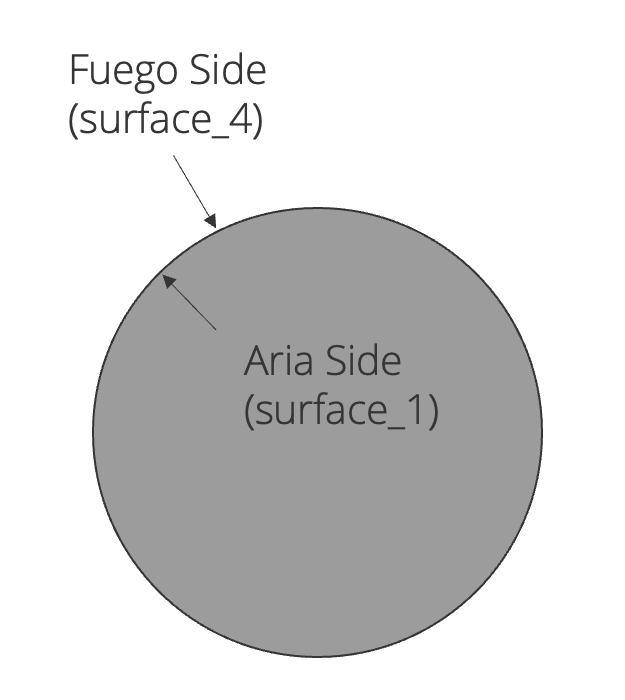
We will need to set up the field transfers between the Fuego surface (surface_4) and the Aria surface (surface_1)

Scope: Procedure

Begin Transfer solid_to_fluid_init
    Interpolate Surface Nodes From Solid_region To Fluid_region
    Send Block surface_1 To surface_4
    Send Field solution->Temperature State Old To Wall_temperature State None
    geometric tolerance = 5e-3
    nodes outside region = abort
End

Begin Transfer fluid_to_solid
    Interpolate Surface Nodes From Fluid_region To Solid_region
    Send Block surface_4 To surface_1
    Send Field flux_linearization_coefficient State None To bc_ref_h State None
    Send Field flux_linearization_temperature State None To bc_ref_temp State None
    geometric tolerance = 5e-3
    nodes outside region = abort
End

Begin Transfer solid_to_fluid
    Interpolate Surface Nodes From Solid_region To Fluid_region
    Send Block surface_1 To surface_4
    Send Field solution->Temperature State New To Wall_temperature State None
    geometric tolerance = 5e-3
    nodes outside region = abort
End

First we must define the transfer blocks. This is split up into three separate blocks. Let’s look at them a bit more closely.

Begin Transfer solid_to_fluid_init
    Interpolate Surface Nodes From Solid_region To Fluid_region
    Send Block surface_1 To surface_4
    Send Field solution->Temperature State Old To Wall_temperature State None
    geometric tolerance = 5e-3
    nodes outside region = abort
End

The solid_to_fluid_init block is the initial transfer between the Aria (solid) surface to the Fuego (fluid) surface. Because these meshes are not contiguous (e.g. the respective surfaces do not share nodes or sides), we use an interpolation transfer, and set a geometric tolerance for said transfer. This is useful in that the meshes between two separate regions can be quite different, where interpolation can handle the mapping from the Aria surfaces to the Fuego surfaces (and vice versa).

Begin Transfer fluid_to_solid
    Interpolate Surface Nodes From Fluid_region To Solid_region
    Send Block surface_4 To surface_1
    Send Field flux_linearization_coefficient State None To bc_ref_h State None
    Send Field flux_linearization_temperature State None To bc_ref_temp State None
    geometric tolerance = 5e-3
    nodes outside region = abort
End

This is the transfer block responsible for transferring fluid (Fuego) fields to the solid (Aria) fields, as we have defined before. The flux_linearization_coefficient and flux_linearization_temperature are automatically computed in fuego for a wall interface boundary (see section Wall). These Fuego fields are sent from surface_4 to the fields bc_ref_h and bc_ref_temp which are on surface_1. Aria will use these fields in the materials and BCs defined in the previous sections.

Begin Transfer solid_to_fluid
    Interpolate Surface Nodes From Solid_region To Fluid_region
    Send Block surface_1 To surface_4
    Send Field solution->Temperature State New To Wall_temperature State None
    geometric tolerance = 5e-3
    nodes outside region = abort
End

This last transfer block sends fields from Aria to Fuego. In this case, Aria is sending the solution->Temperature field to the Fuego Wall_temperature field which will be used as a boundary condition in Fuego.

5.1.4.3.6. Coupling Fuego and Aria

Solution control lets us control when Fuego and Aria are executed, when transfers happen, and when overall nonlinear convergence is met for a time step.

Begin Solution Control Description
  Use System Main

  Begin Initialize Mytransient_init
      Advance Fluid_region
      Advance Solid_region
      Transfer solid_to_fluid_init
  End

  Begin System Main
    Use Initialize Mytransient_init

    Begin Transient Mytransient
      Begin nonlinear CHT
        Advance Fluid_region
        Transfer fluid_to_solid
        Advance Solid_region
        Transfer solid_to_fluid
      End
    End
  End

  Begin Parameters for Nonlinear CHT
    Converged when "(Fluid_region.MaxInitialNonlinearResidual(0) < 1E-1 &&  \$
                      Solid_region.MaxInitialNonlinearResidual(0) < 1E-2) || \$
                      CURRENT_STEP > 1"
  End
End

Now that we have two regions, we want to set up a solution control description that will advance both regions and do the appropriate field transfers. First we have

Begin Initialize Mytransient_init
    Advance Fluid_region
    Advance Solid_region
    Transfer solid_to_fluid_init
End

Which uses the initialization transfer block shown in the previous section. First we initialize the fluid region, the solid region, and then do the transfer from solid to fluid (Aria to Fuego). This ensures that for the first actual time step, Fuego has a non-zero wall temperature.

Next we need to set up a nonlinear loop for the time stepping, and some convergence criteria

Begin System Main
  Use Initialize Mytransient_init

  Begin Transient Mytransient
    Begin nonlinear CHT
      Advance Fluid_region
      Transfer fluid_to_solid
      Advance Solid_region
      Transfer solid_to_fluid
    End
  End
End

Begin Parameters for Nonlinear CHT
  Converged when "(Fluid_region.MaxInitialNonlinearResidual(0) < 1E-1 &&  \$
                    Solid_region.MaxInitialNonlinearResidual(0) < 1E-2) || \$
                    CURRENT_STEP > 1"
End

The nonlinear loop will continue to execute until the prescribed convergence criteria is satisfied. This corresponds to the coupling algorithm we outlined at the beginning of this tutorial.

Setting up the time stepping parameters is the same as in the previous tutorials, but now we must supply parameters for both the Aria (solid) and Fuego (fluid) regions

#-------------------------------------------
Begin Solution Control Description
  ...

  Begin Parameters For Transient Mytransient
      Start Time       = 0.0
      Initial Deltat   = 0.1
      Termination Time = 10.0
$-----------------------------------------------------
$               Define Fuego time integration settings
$-----------------------------------------------------
      Begin Parameters For Fuego Region Fluid_region
        Transient Step Type Is Automatic
        Cfl Limit = 5.0
        Time Step Change Factor = 1.5
      End   Parameters For Fuego Region Fluid_region
$-----------------------------------------------------
$               Define Aria time integration settings
$-----------------------------------------------------
      Begin Parameters For Aria Region Solid_region
        Initial Time Step Size = 0.1
        Time Step Variation = Adaptive
        Predictor-corrector Tolerance = 1.0e-3
        Time Integration Method = BDF2
      End   Parameters For Aria Region Solid_region
  End   Parameters For Transient Mytransient

Here, we specify a CFL limit for the automatic time stepping in the Fuego region. In the Aria region, we also set an adaptive time step tolerance with a 2nd order time stepping method. For more information on setting up the transient parameters in Aria, please see the Aria User Manual.

5.1.4.4. Running Aria/Fuego and Reading The Logfile

To run the coupled simulation, open a terminal and navigate to where your input files and mesh files are located, and run the following commands:

module load sierra
mpirun -n 4 aria_fuego -i flow_over_cylinder_cht.i

A typical time step in a coupled simulation is shown here

-------------- For equation system name: main --------------
Global predictor error = 4.245e-07
Time step selection: dt <= 8.734e-01 (based on Predictor-Corrector Tolerance).
Time step selection: dt <= 7.224e-02 (based on Maximum Time Step Size Ratio).
Time step selection: dt <= 1.798e+308 (based on Maximum Time Step Size).
Time step selection: dt <= 8.720e-02 (based on Stability limit for dt Ratio).
Time step selection: dt  = 7.224e-02 (Adaptive time stepping result).
Global Variable Value
--------------- -----
Region::execute() time for Solid_region: 1.994e-02 sec.
Transfer Solid_To_Fluid, time 2.578, time step 0.03612
  Fluid_region.MaxInitialNonlinearResidual:
    system -> X_Momentum : 1.59529e-07
    system -> Y_Momentum : 1.15093e-07
    system -> Continuity : 2.06795e-07
    system -> Turbulent_Kinetic_Energy : 2.9319e-09
    system -> Enthalpy : 0.0339821
  Fluid_region.MaxInitialNonlinearResidual() = 0.0339821
  Solid_region.MaxInitialNonlinearResidual:
    system -> main : 3.702e-06
  Solid_region.MaxInitialNonlinearResidual() = 3.702e-06
Minimum Time Step Selection:
        min           max
    0.000e+00     3.611e-02     Fluid_region
    1.000e-16     7.224e-02     Solid_region
    0.000e+00     3.611e-02     CHT
Transient Mytransient: dt = 0.03611
Transient Mytransient, step 67, time 2.6144e+00, time step 3.6106e-02, 26.14% complete

A couple of things to note here is the CHT residual summary. Here we show that Fluid_region.MaxInitialNonlinearResidual and Solid_region.MaxInitialNonlinearResidual are both within the acceptable tolerance, so the coupled solution is converged. The timestep is chosen such that the minimum allowable timestep between both regions is selected. In this case, the Fluid_region is selecting the next timestep based on the CFL condition.

5.1.4.5. Viewing Results

Please follow the steps from the previous tutorial to run ParaView Viewing Results.

First lets visualize the fluid domain temperature.

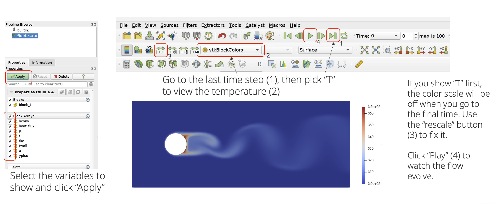
Notice that since we have only loaded the Fuego results exodus file, we only see the Fuego region of the flow field. Let’s load the solid (Aria) region in the same view.

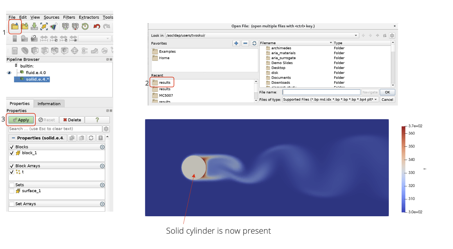
Now we can see the solid region cylinder, we can then color it by temperature as well.

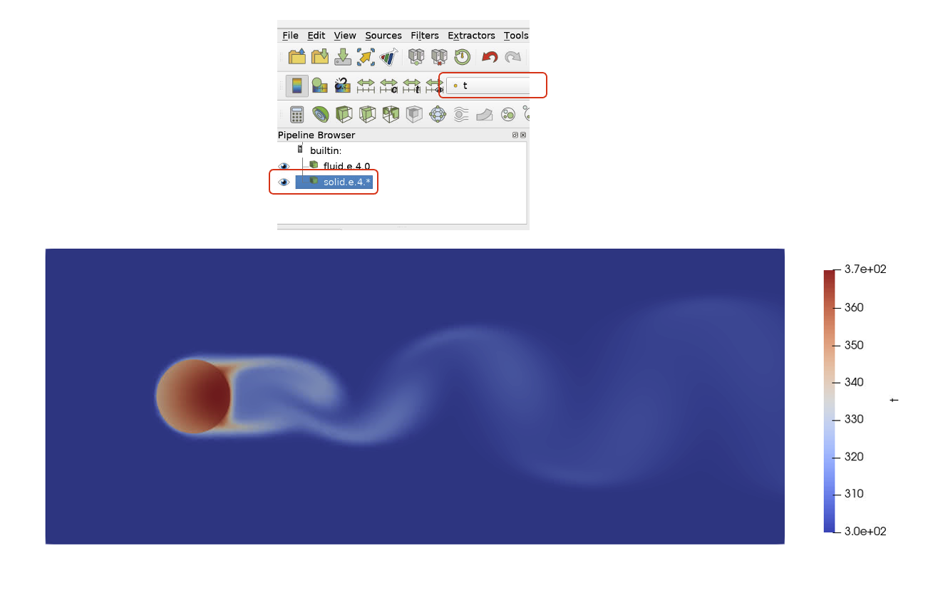
Now we have a full picture of the temperature field on both the solid and fluid domains. Notice that the temperature inside the cylinder is lower at the leading edge compared to the trailing edge. This is an effect of the convective cooling of the relatively cold fluid temperature on the relatively hot solid temperature. Notice how the temperature of the trailing vortices changes as it travels downstream.

Let’s observe the convective coefficient and how it changes with time.

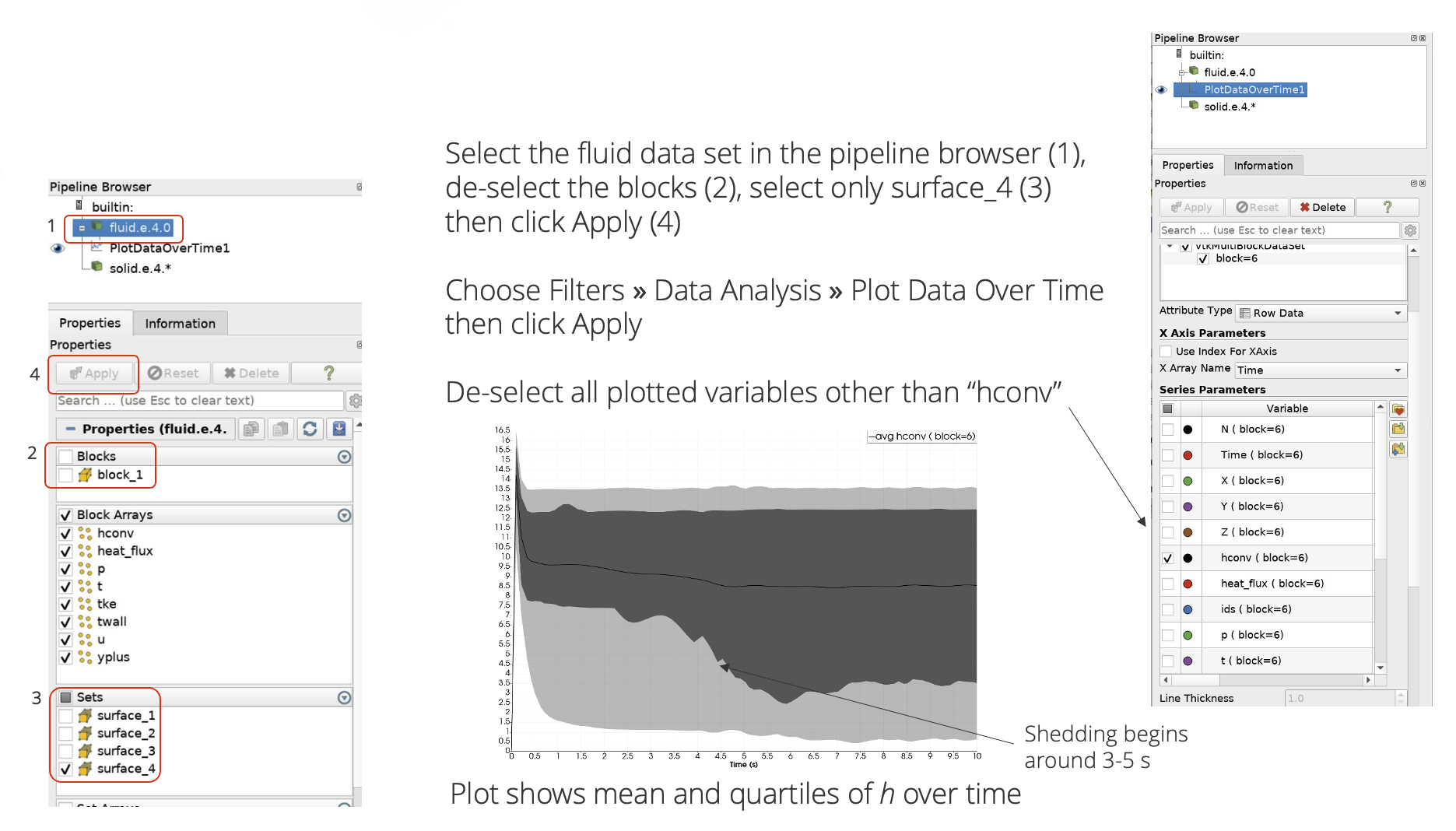
Here we can see how the global convective coefficient changes with time. When the vortex shedding starts, how does the convective coefficient behave? Is this expected?