Curved Surface Friction Behavior
Product: Sierra/SolidMechanics - Explicit Analysis
Problem Description
The purpose of this problem was to examine the frictional contact behavior of explicit analysis in Sierra, specifically that of curved contact surfaces. The scenario of this problem was this: a cylindrical mass is placed atop a slope of a given angle and allowed to roll down it. As it rolls, slip may occur at the contact surface if the frictional force is not large enough compared to the cylinder’s acceleration along the slope. Naturally, when the slope is horizontal or almost horizontal, the cylinder should “stick” to the surface and roll without slipping if it rolls at all, but when the slope is oriented near vertical, the cylinder should hardly spin at all, and will experience large slip values as it moves along the surface. With this in mind, the slip at the contact surface was measured for several slope angles and several frictional coefficients, then compared to ideal behavior to determine the accuracy of the frictional model (Fig. 50).
Mesh Model Setup
The cylinder was modeled with a radius of 0.2m, and a length of 0.2m. A conversion study was performed to determine when the model mesh was fine enough that the slip data obtained from the model had begun to converge on an accurate solution without requiring undue processing time. The results are shown in Fig. 46, and a mesh refinement level of 5 was used as a result. Note: the mesh refinement level refers to the auto size setting in Cubit’s meshing commands. The slope was modeled as a rectangular block 10m long, 0.5m wide, and 0.1m thick. Mesh elements were chosen as 0.1m cubes to balance the need for a fine mesh with the need for fast run times (Fig. 47).
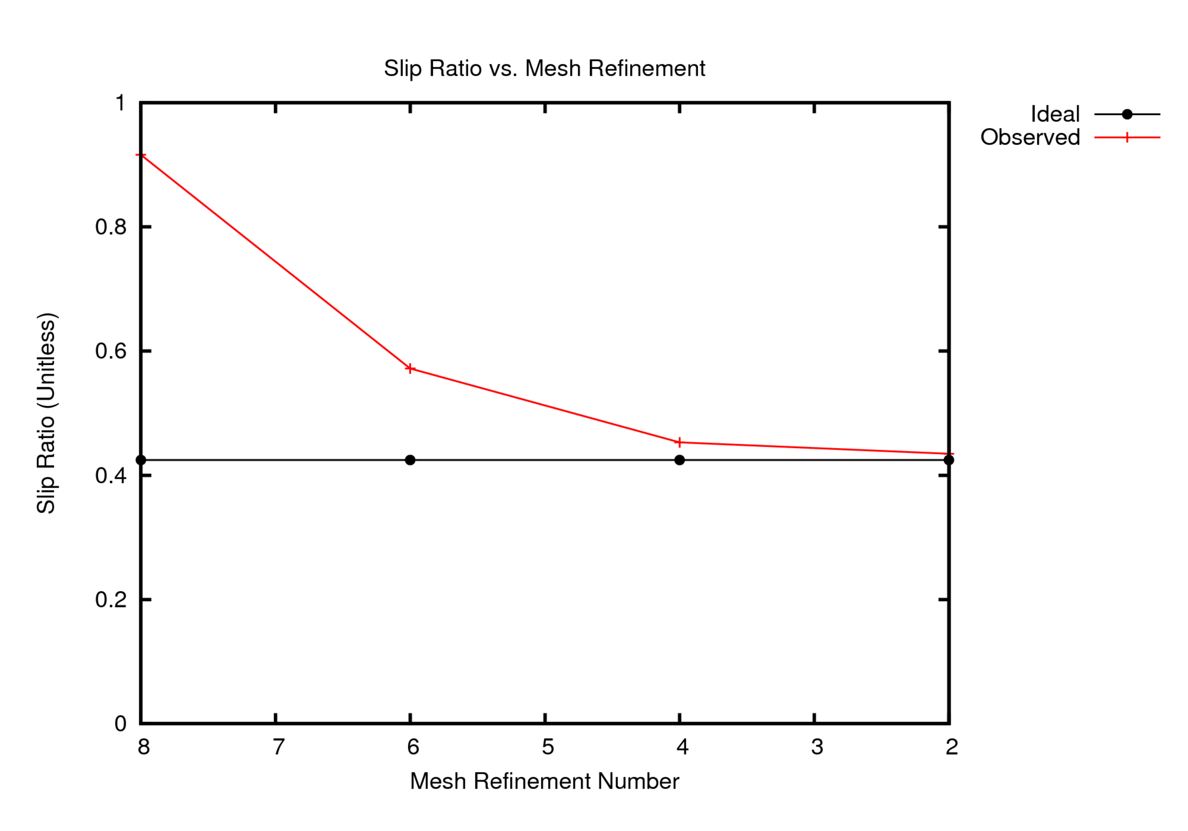
Fig. 46 Mesh Convergence
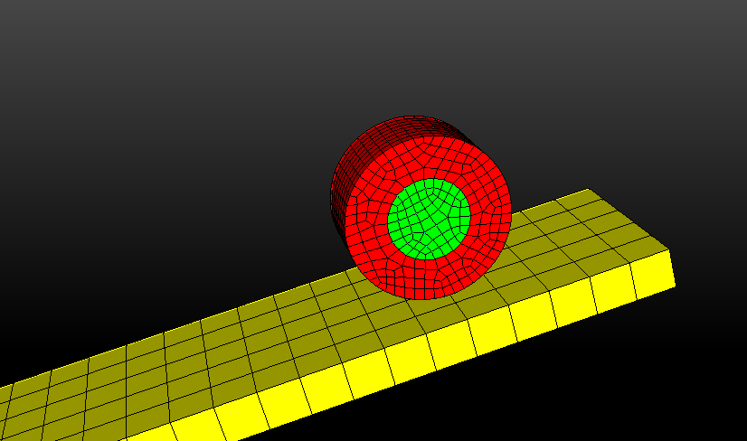
Fig. 47 Mesh Refinement
Boundary Conditions and General Problem Setup
The slope was constrained to zero displacement in each direction, while the cylinder had no constraints on its movement, and was introduced with zero initial velocity. Because the rotational velocity of the cylinder was needed to determine its slip magnitude, it was first modeled as a rigid body to access the rigid body output variables. This resulted in poor results at friction coefficients above 0.25 (Fig. 48), so the cylinder was instead modeled as a non-rigid cylinder with a rigid body core that had been merged with it. This resulted in more accurate results across the spectrum of examined friction coefficients, especially at higher settings (Fig. 49). Note: The slope and cylinder were not part of the same block entity. The slope was not modeled as a rigid body, but due to its zero displacement boundary condition, it did not deform or experience stresses anywhere.

Fig. 48 Rigid Body Contact |
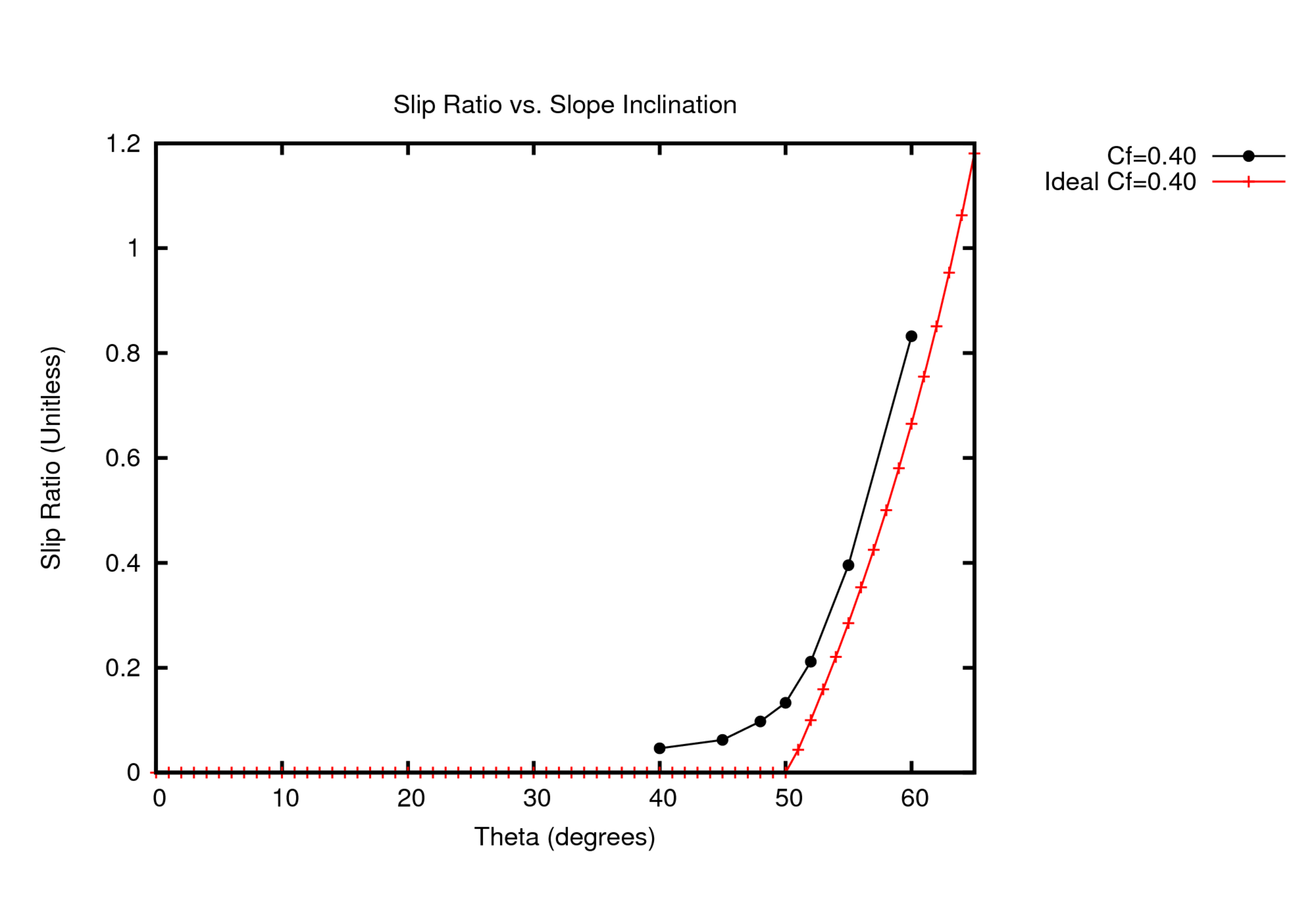
Fig. 49 No Rigid Body Contact |
Metric units are used |
|---|
Displacement: meters |
Mass: kilograms |
Time: seconds |
Force: \(kgm/s^2\) |
Temperature: Kelvin |
Young’s Modulus |
E |
\(68.9\times10^9\) |
Poisson’s Ratio |
\(\nu\) |
\(0.3333\) |
Density |
\(\rho\) |
\(2720\) |
Yield Stress |
\(\sigma_{yield}\) |
\(276\times10^6\) |
Hardening Modulus |
H |
0.0 |
Contact was enforced as general contact with “skin all blocks” set to on. Gravity was enforced as a constant of \(9.81m/s^2\) in the negative y direction. Friction was modeled as a constant coefficient of friction which varied from test to test. Slope angle was determined by rotating both volumes in cubit by a prescribed angle.
Feature Tested
Curved surface frictional contact behavior.
Ideal Behavior Model
Ideal behavior was based on a basic physics model manually calculated as shown.
Nomenclature |
|||||
|---|---|---|---|---|---|
Friction Coefficient |
(\(C_{f}\)) |
Translational Velocity |
(\(V\)) |
Normal Force |
(\(f_{N}\)) |
Slope Angle |
(\(\theta\)) |
Translational Acceleration |
(\(a\)) |
Frictional Force |
(\(f_{f}\)) |
Gravitational Constant |
(\(g\)) |
Rotational Velocity |
(\(\omega\)) |
Gravitational Force |
(\(f_{g}\)) |
Cylinder Rotational Inertia |
(\(I\)) |
Rotational Acceleration |
(\(\alpha\)) |
||
Mass of Cylinder |
(\(m\)) |
Slip Ratio |
(\(S_{R}\)) |
||
Radius of Cylinder |
(\(r\)) |
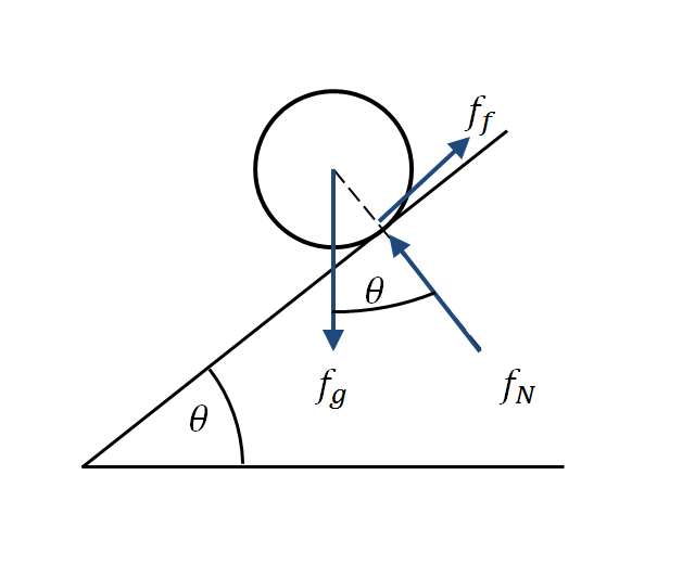
Fig. 50 Basic Physics Model
a
(7)\[S_R = \frac{V}{\omega r} - 1 .\](8)\[S_R\neq0\; \; iff\; \; \alpha r \neq a .\](9)\[\alpha = \frac{f_f r}{I} = \frac{2f_f}{m r} .\](10)\[I=\frac{1}{2} m r^2 .\](11)\[f_f=C_f f_N=C_f f_g cos(\theta) .\](12)\[a=(f_gsin(\theta)-f_f)/m=f_g(sin(\theta)-C_f cos(\theta))/m .\](13)\[\therefore \alpha r = a \; \; \; \; \; becomes: \; \; \; \; 2r(\frac{C_f f_g cos(\theta)}{m r})=f_g \frac{sin(\theta)-C_f cos(\theta)}{m} .\](14)\[\therefore\; , \;S_R = 0 \; \; \; \; \; when \; \; \; \; \; \theta <= tan^{-1}(3C_f) .\]
This establishes that there is a threshold beyond which the frictional force cannot overcome the gravitational force in the direction of motion. This threshold is defined as: \(\theta=tan^{-1}(3C_{f})\).
After the threshold has been reached, slip occurs. To measure slip relative to velocity, the slip ratio (\(S_R\)) is defined as \(S_{R}=V/(\omega * r) - 1\), and is positive when the cylinder’s tangential velocity is less than its translational velocity (\(\omega*r<V\)). The ideal slip ratio behavior was calculated as:
The slip ratio does not vary with time as the cylinder moves down the slope, establishing an ideal case to rate results from the analysis.
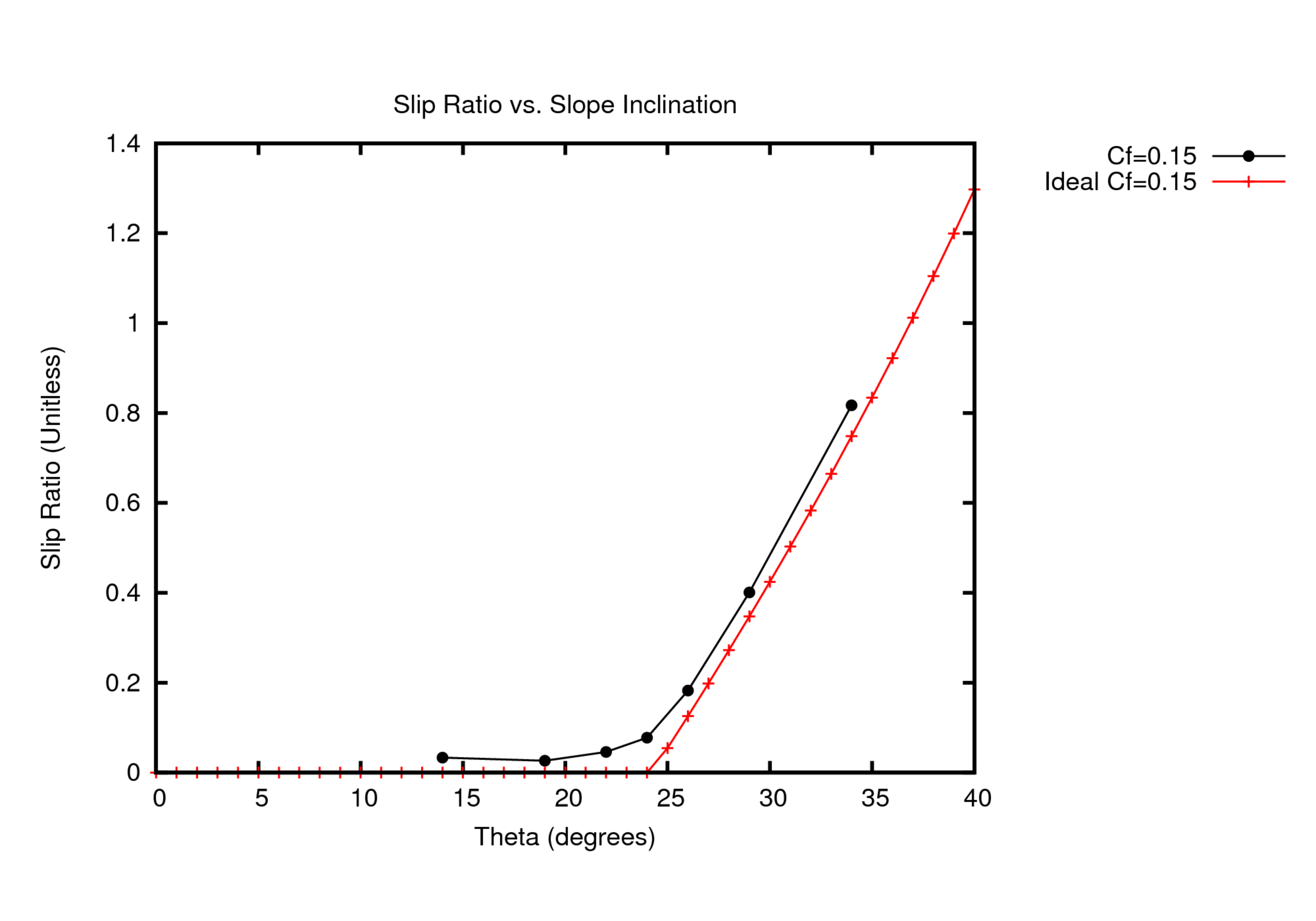
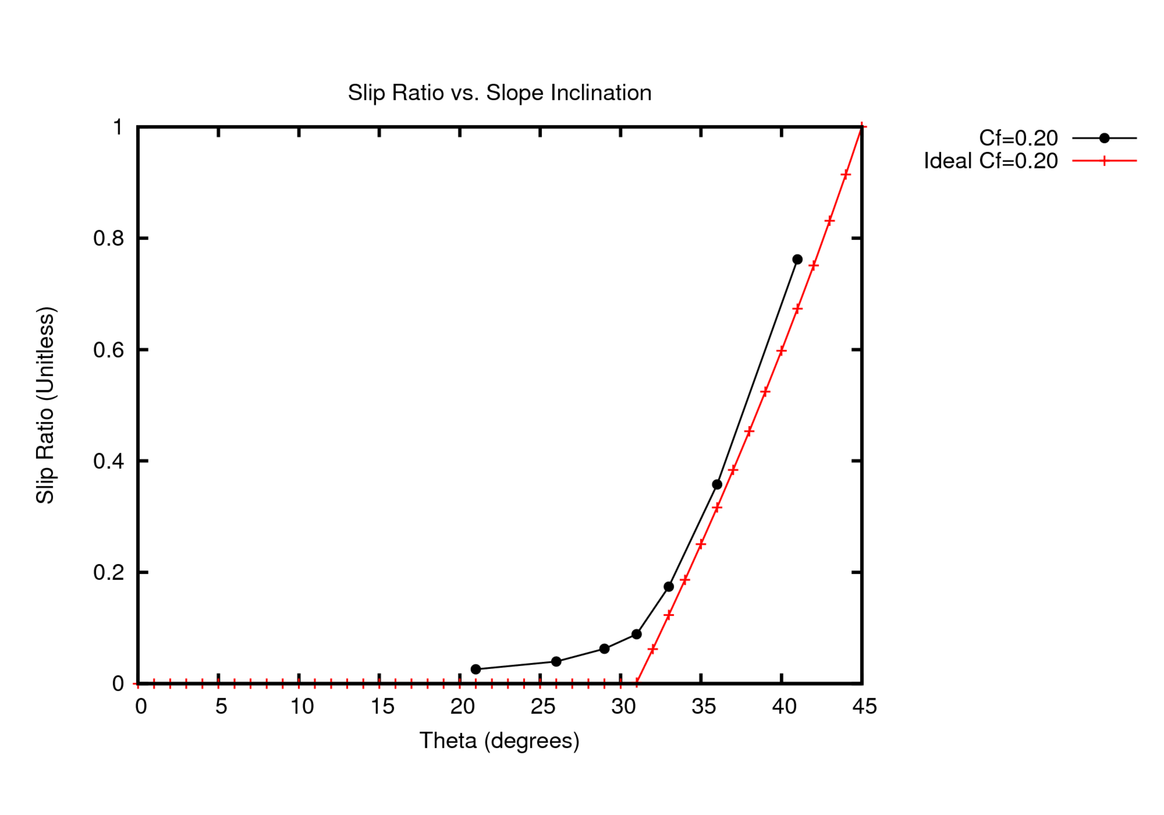
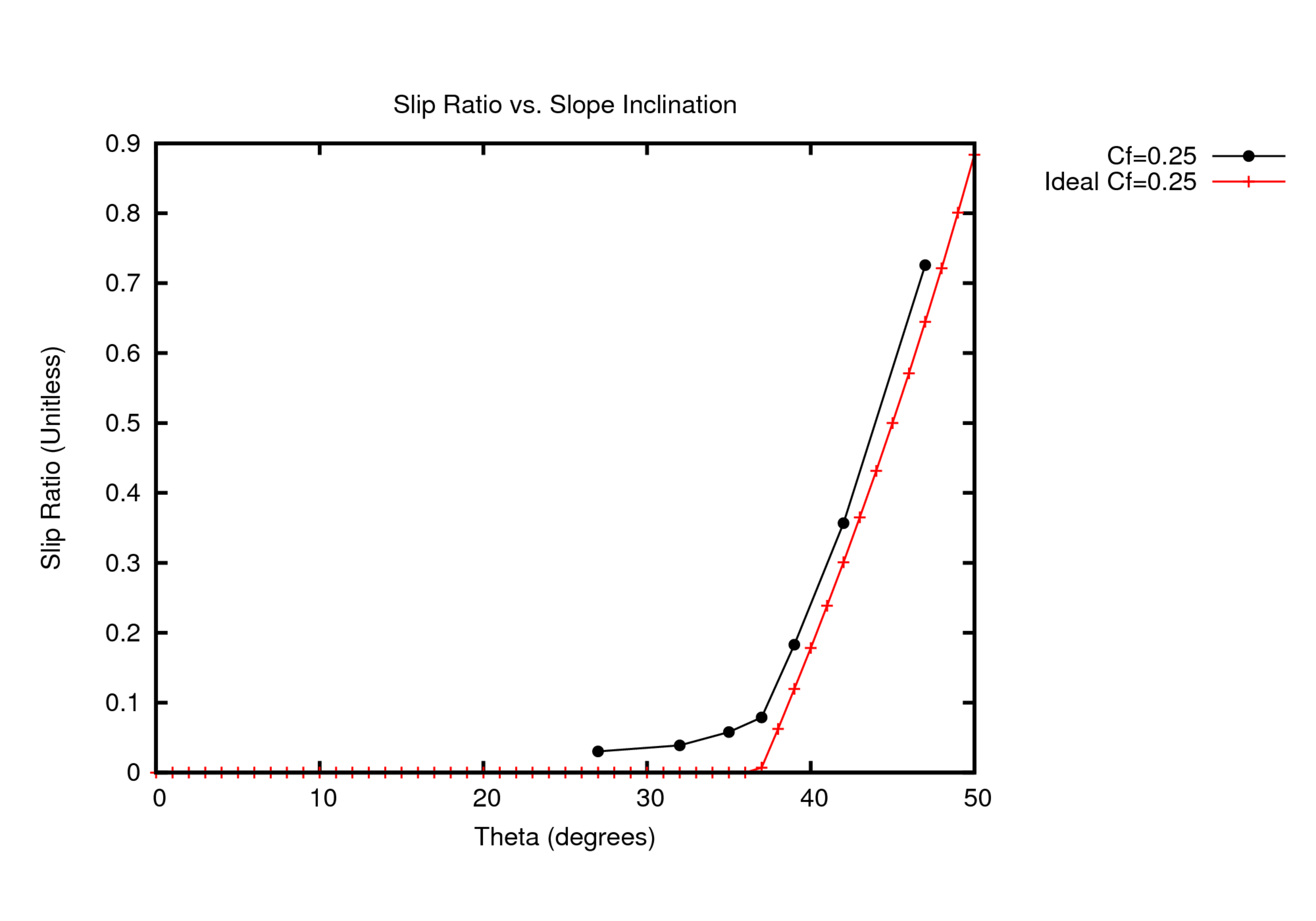
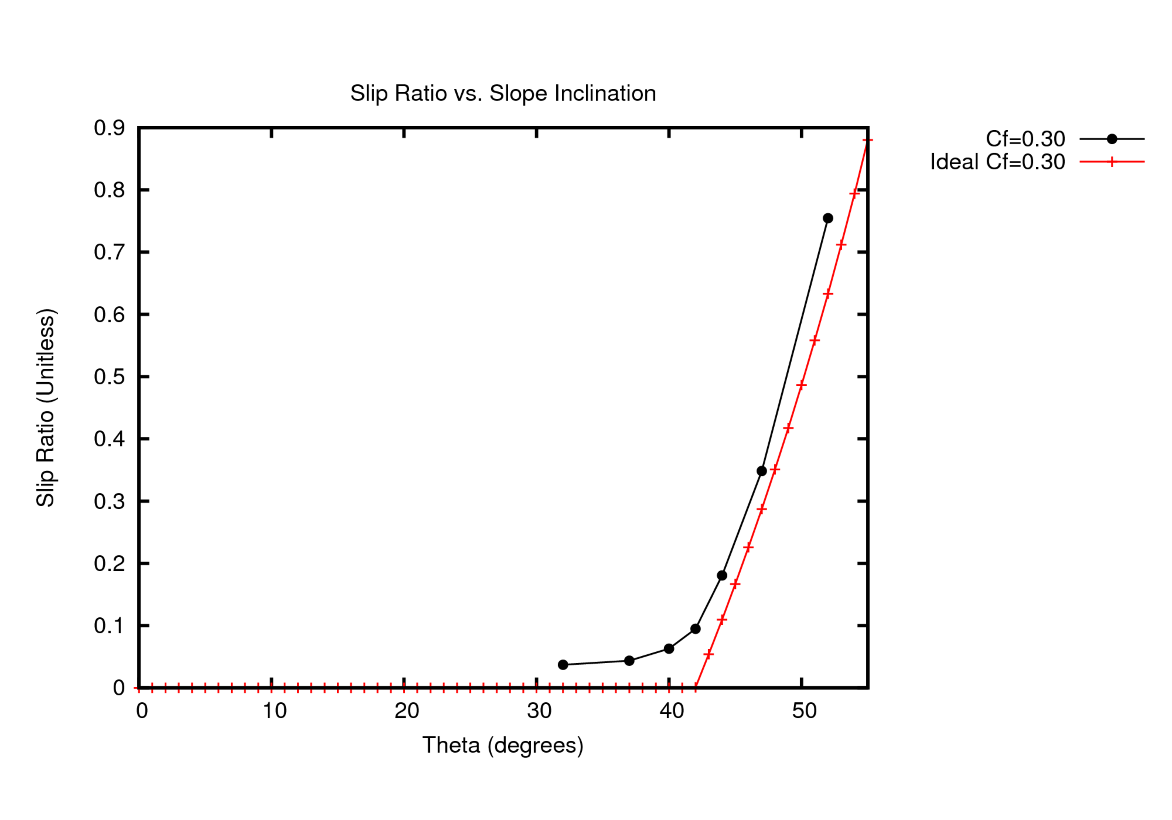
Results and Discussion
The following graphs show the slip ratios of various frictional coefficients near their respective threshold angles, shown side by side with their ideal behavior. Figures(Fig. 52) show the observed and ideal behavior of each friction coefficient, consolidated into Fig. 51 a and Fig. 51 b. Note: Each data point represents a separate simulation.
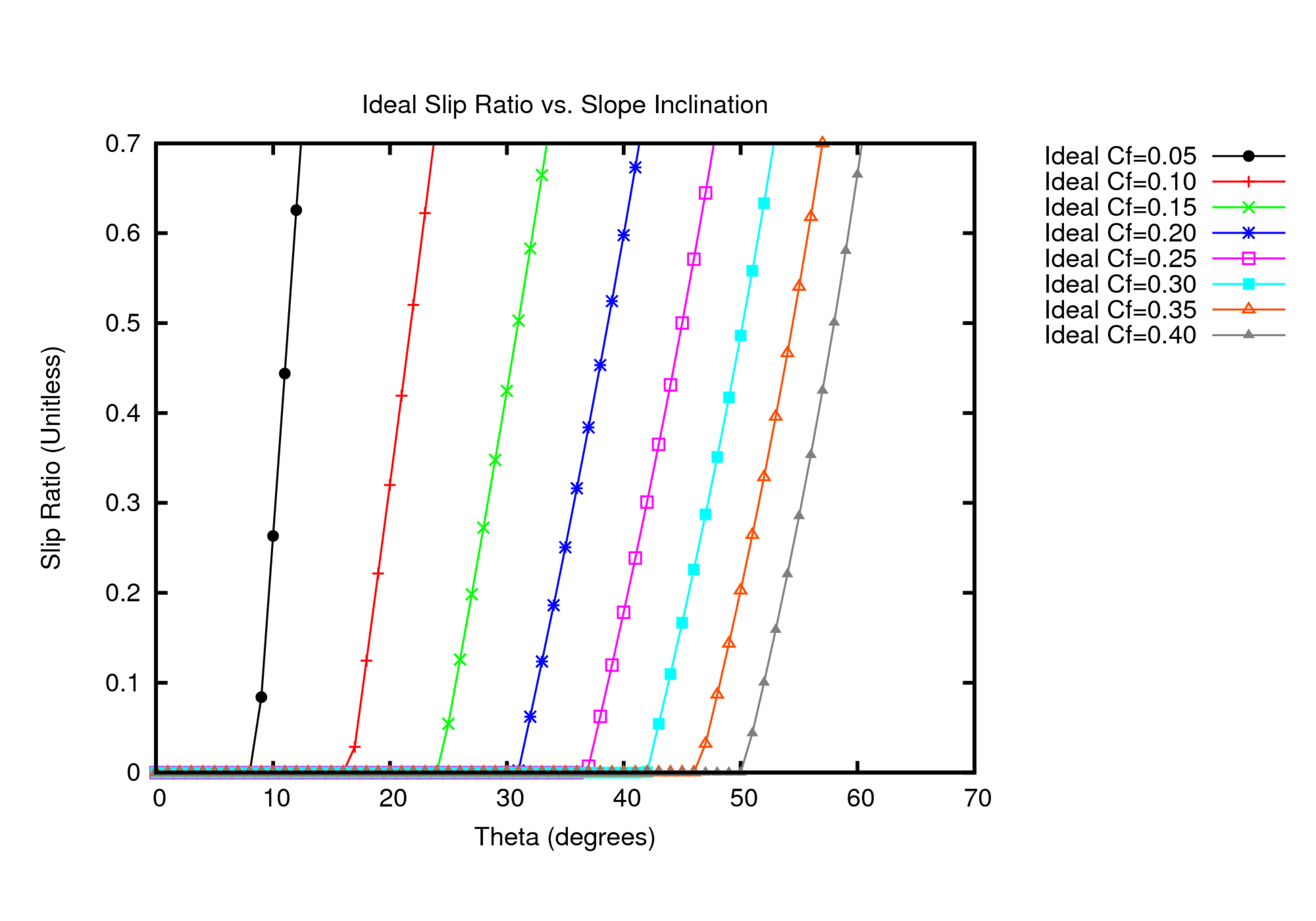 Predicted Slip
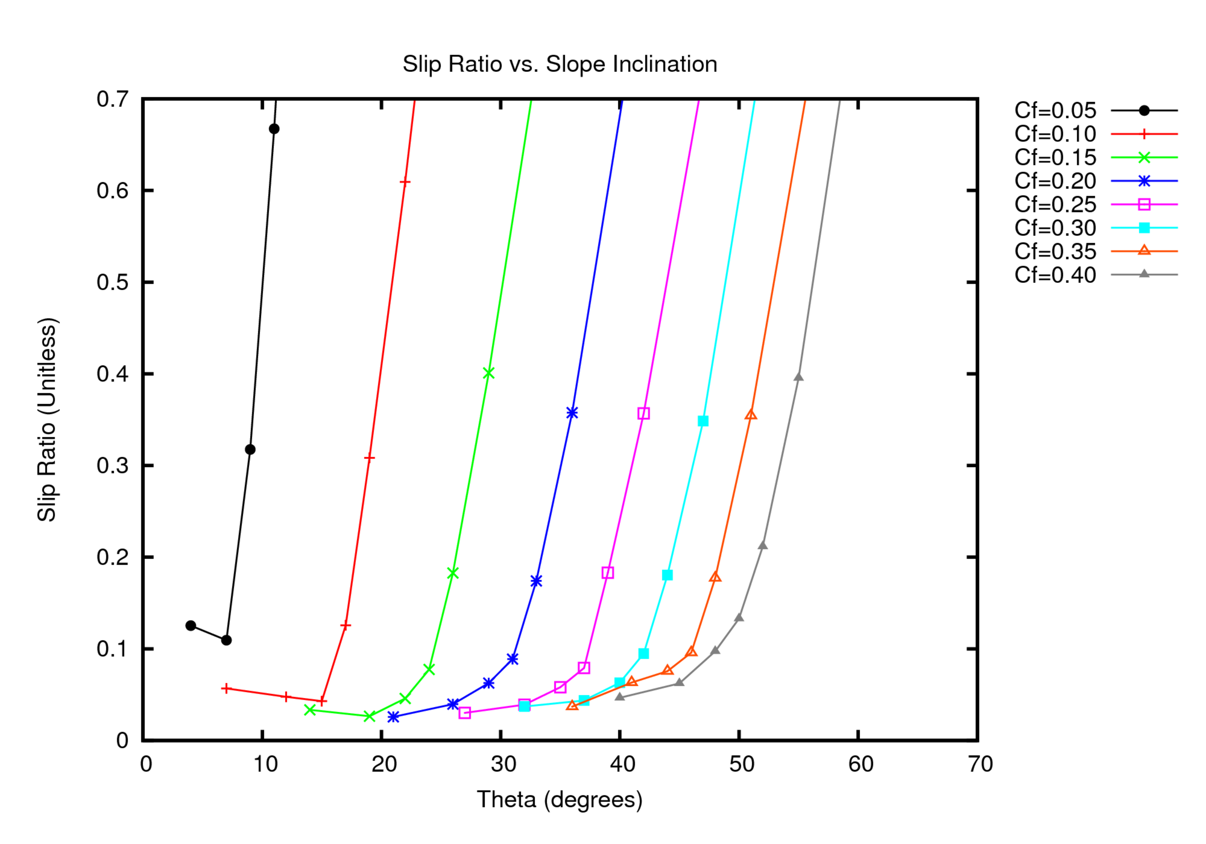 Observed Slip
Fig. 51 Slip ratios
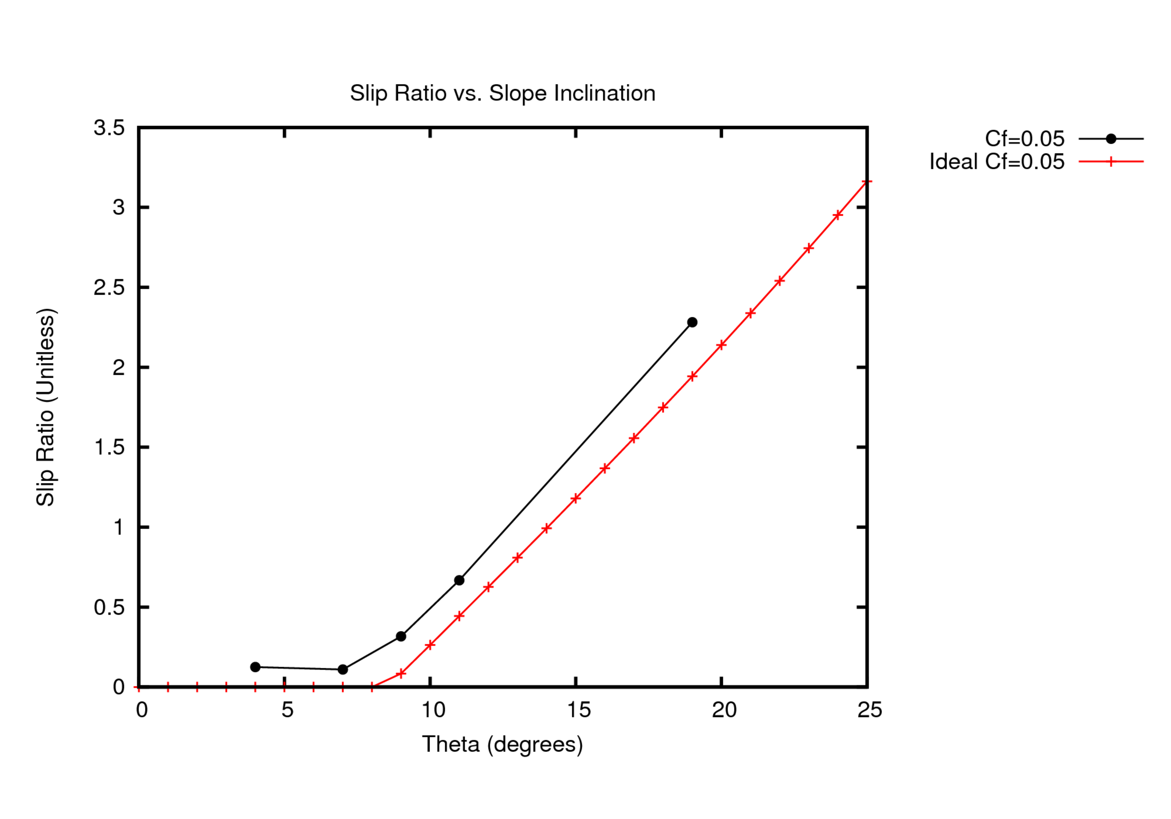 Coefficient = 0.05
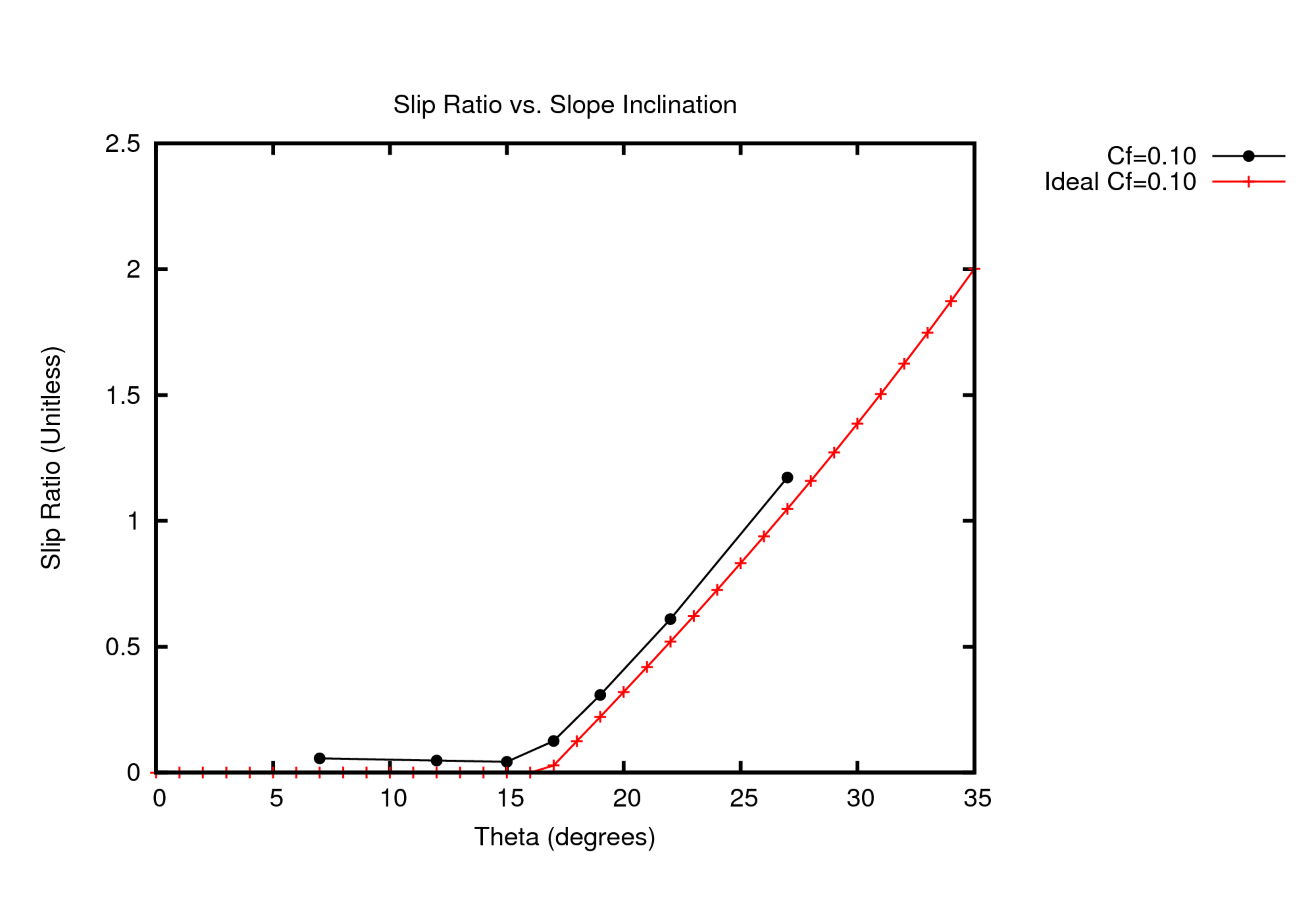 Coefficient = 0.10
 Coefficient = 0.15
 Coefficient = 0.20
 Coefficient = 0.25
 Coefficient = 0.30
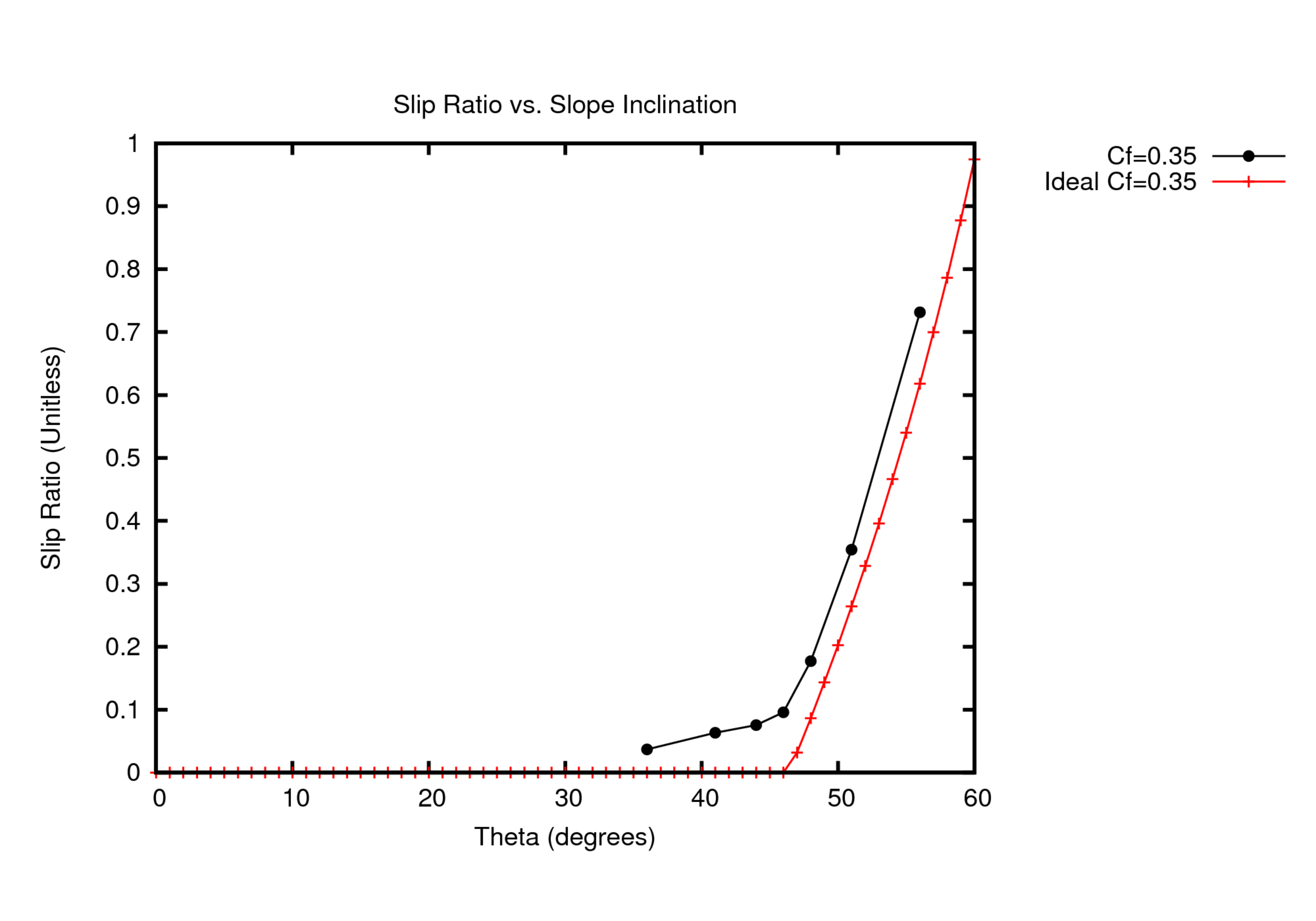 Coefficient = 0.35
Coefficient = 0.40
Coefficient = 0.35
Coefficient = 0.40
Fig. 52 Various frictional coefficients’ response and respective threshold angles
Conclusion
Frictional contact with curved surfaces appears to behave as expected in explicit analysis, with results that converge to the ideal solution as mesh refinement increases. Defining an interior volume as a rigid body successfully produces accurate results without restricting access to rigid body output variables such as angular velocity.