Ball Bearing Pull

Product: Sierra/SolidMechanics - Implicit Analysis

Problem Description

The purpose of the following example is to demonstrate three different ways of solving a complicated preload problem: via implicit statics and using the FETI linear solver as the preconditioner, via implicit statics and using the nodal preconditioner, and via explicit quasistatic mode. The results of all methods are compared and the input file options are discussed in the Results and Discussion Section.

The geometry consists of a simple housing with eight ball ball bearings inside and a shell “cage” is used to lock the balls into place. The inner race of the housing is pulled axially upward while the outer race is held fixed. The initial configuration of the problem can be seen in Fig. 59.

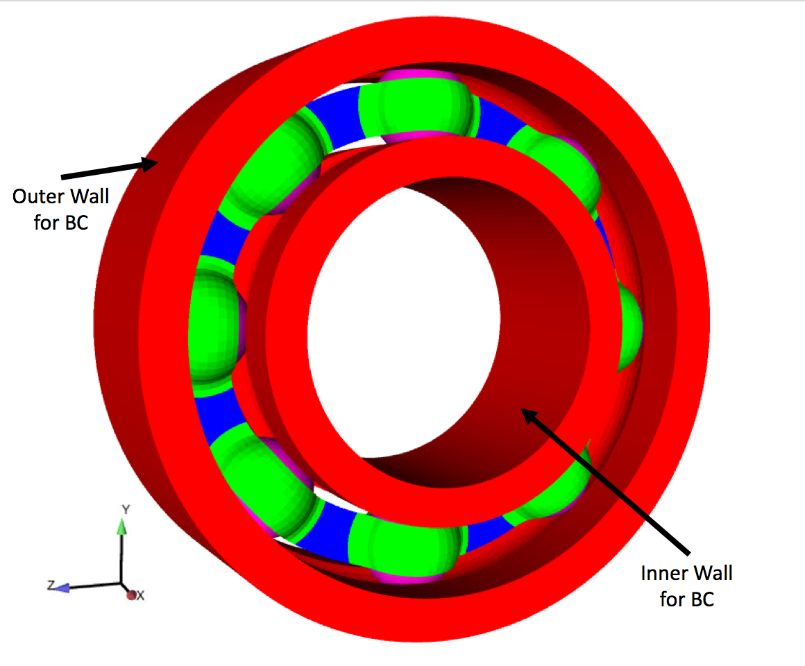
Fig. 59 Initial Problem Geometry

Loading and Boundary Conditions

The outer wall of the housing is fixed in the X direction, in the radial X direction (via the prescribed BC of zero), and in the cylindrical X direction (via the prescribed BC of zero). A prescribed displacement is applied to the inner wall of the inner race in the X direction via a linear ramp function. This same surface is also fixed in the radial X direction and in the cylindrical X direction (via the prescribed BC of zero).

Material Model

An elastic material model is used for all blocks. The housing and the ball bearings are modeled using Stainless Steel 440C material properties. The shell cage is modeled using Stainless Steel 305 material properties.

Details of the material properties can be seen in the below table:

Metric units are used
Displacement: meters
Mass: kilograms
Time: seconds
Force: \(kgm/s^2\)
Temperature: Kelvin

Table 16 Stainless Steel Material Properties

Stainless Steel
Young’s Modulus: Stainless Steel 440C	E	\(3.04*10^7\)
Young’s Modulus: Stainless Steel 305	E	\(2.80*10^7\)
Poisson’s Ratio	\(\nu\)	\(0.283\)
Density: Stainless Steel 440C	\(\rho\)	\(7.30*10^3\)
Density: Stainless Steel 350	\(\rho\)	\(7.49*10^3\)

Finite Element Model

Standard uniform gradient hexahedral elements were used for the ball bearings and the housing. The default quadrilateral shell element was used for the cage (Belytschko-Tsay).

Feature Tested

The following features are used for all problems: Frictional contact, prescribed boundary conditions, shell/solid contact, shell lofting, user output, quasistatic mode,

The following features are used for the explicit version of the problem: Quasistatic mode

The following features are used for the implicit version of the problem that uses the nodal preconditioner: Nodal probe preconditioner, energy reference, Lagrange adaptive penalty = uniform, adaptive time stepping, corner algorithm = 14.

The following features are used for the implicit version of the problem that uses the FETI preconditioner: Full tangent preconditioner (using FETI as the linear solver), tangent diagonal scale, minimum updates for loadstep, minimum convergence rate, energy reference, Lagrange adaptive penalty = uniform, adaptive time stepping, corner algorithm = 14.

Results and Discussion

Figures Fig. 61 , Fig. 62, and Fig. 63, show the Force-Displacement curves for each of the approaches used. Fig. 64 shows all of the force-displacement curves overlaid on the same plot.

As can be seen in the plots, the two implicit solutions lie on top of each other, while the explicit-quasistatic solution exhibits high frequency oscillations. This is due to the explicit solver having no convergence tolerance within the step, leading to drift in the solution that is correct later in the simulation. The smoother response of the implicit analyses results from the analysis converging to the residual tolerance (in this case, the energy balance is less than or equal to 1.0e-8 or the relative change in the energy balance is less than 1.0e-5). This means that the system is brought into equilibrium after each time step. This example illustrates using explicit quasistatic mode can always get a preload solution, but that solution may be very different than the actual converged statics solution. Therefore, it is almost always worth the effort to put in the extra time to get a preload problem to solve implicitly.

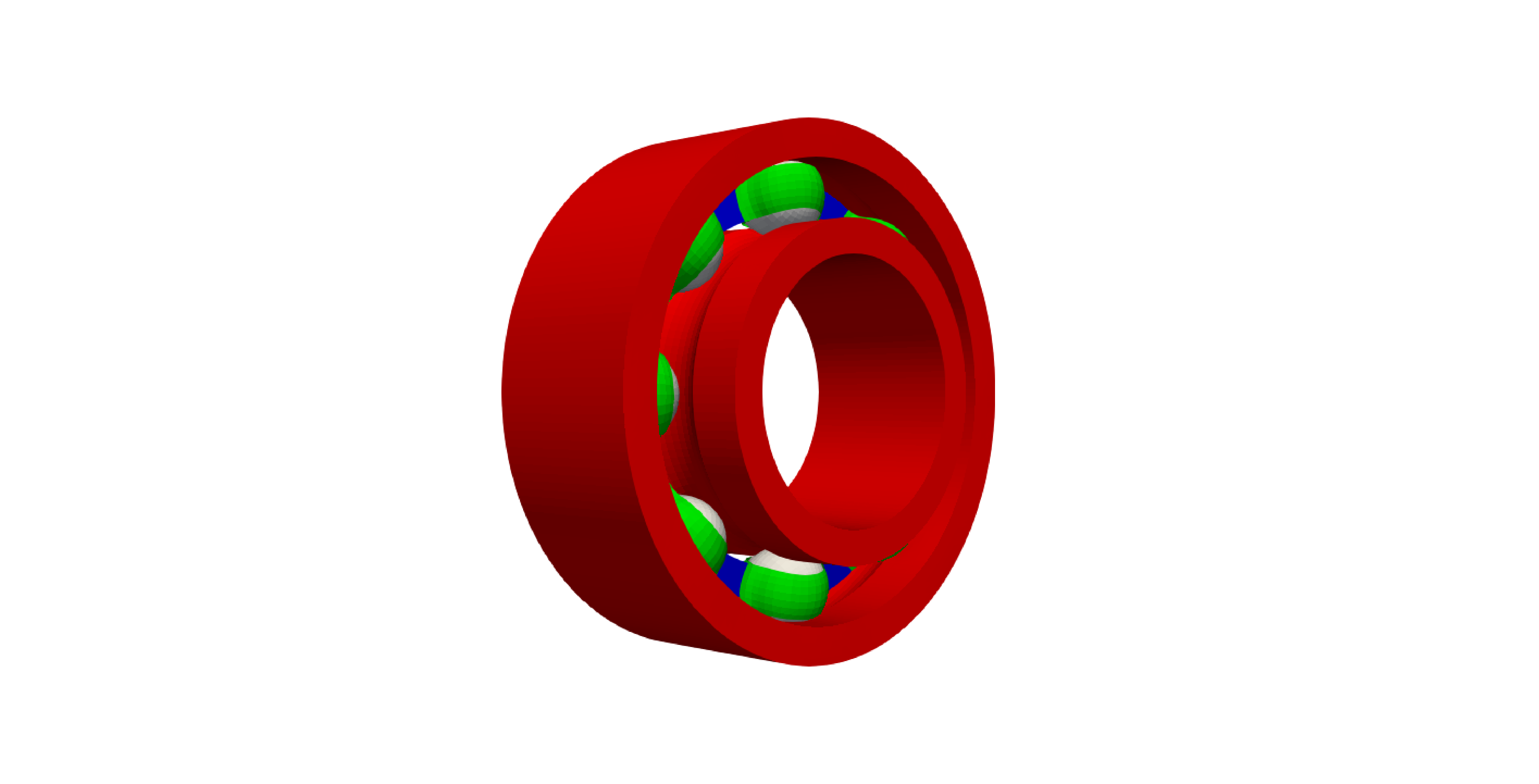
Fig. 60 Geometry after loading

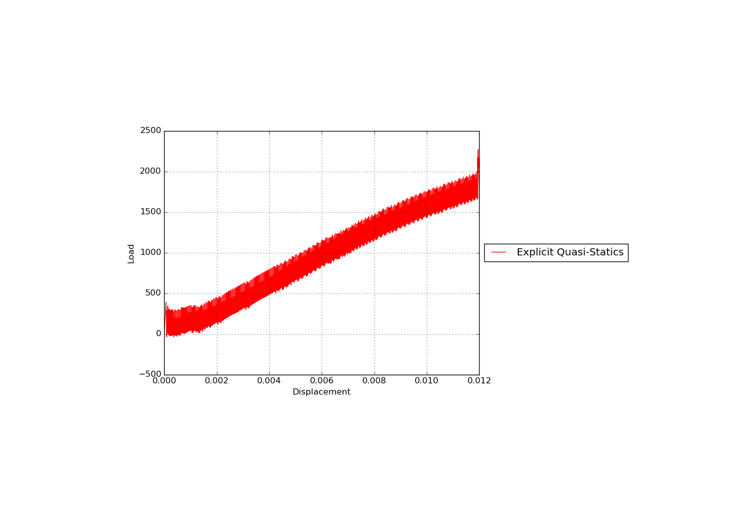
Fig. 61 Force-Displacement curve for Explicit Quasi-Static analysis

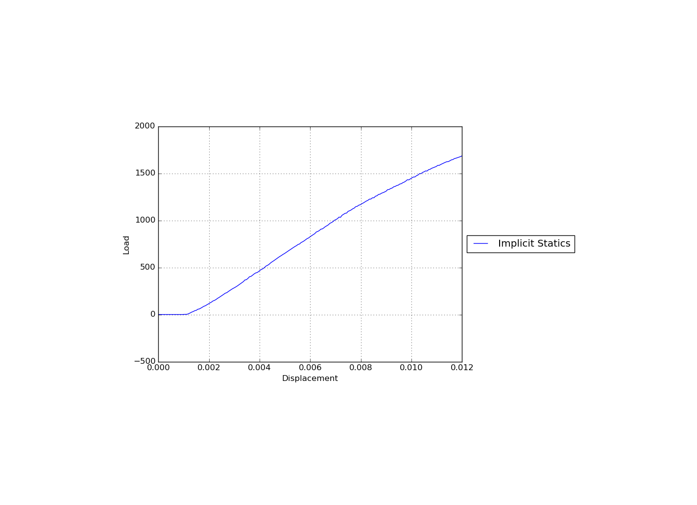
Fig. 62 Force-Displacement Curve for Implicit Statics analysis

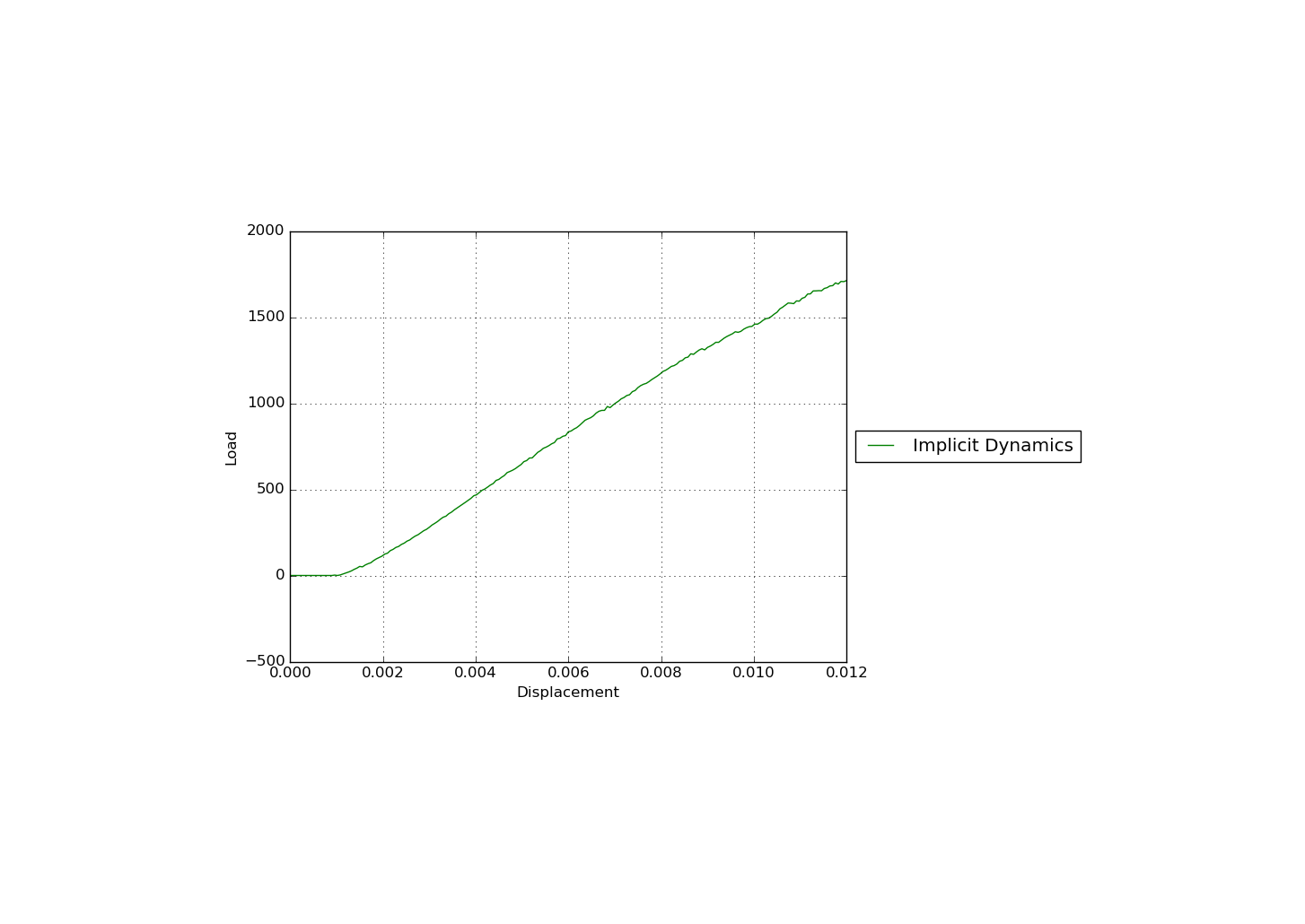
Fig. 63 Force-Displacement Curve for Implicit Dynamic analysis

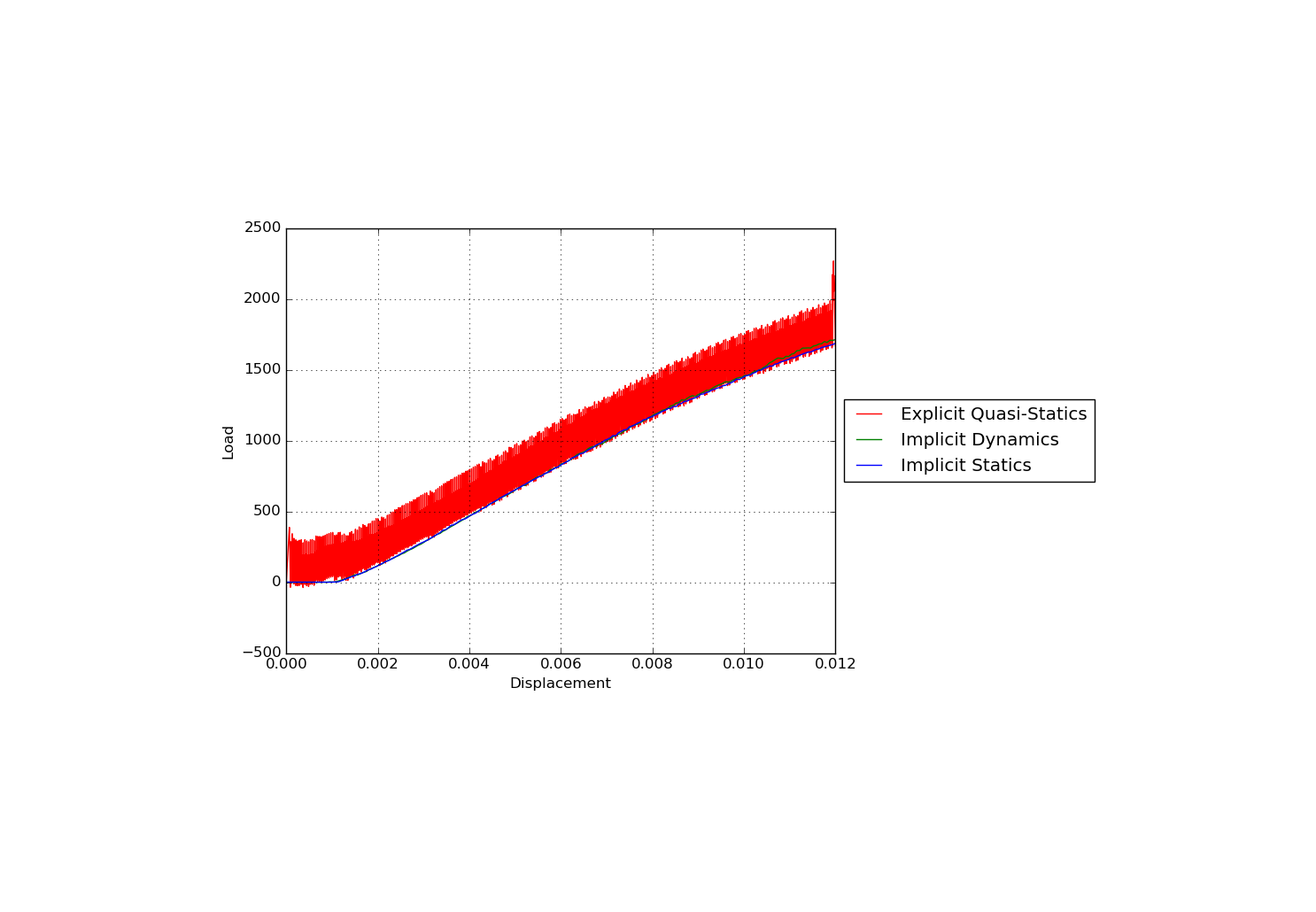
Fig. 64 Comparison of Explicit and Implicit Solutions

Solver Settings Discussion

1. Using the energy reference instead of the external reference. When solving implicit contact problems, using the option REFERENCE = ENERGY usually converges much better than using the external force reference.

2. Using adaptive time stepping with a large number of failure cutbacks and target iterations.

3. When using FETI and the Full Tangent Preconditioner, using corneralgorithm = 14 in FETI. This puts the contact nodes in the coarse grid, keeping FETI from finding rigid body modes on the contact nodes.

4. Adding a small amount of tangent diagonal scale (to help eliminate rigid body modes).

5. Setting maximum updates for loadstep to 0 for performance.

6. Setting minimum convergence rate to 0.1.

Files

• Mesh

• Feti Input Deck

• Nodal Input Deck

• Explicit Quasistatic Input Deck