4.1. Multilevel Solver

Sierra/SM allows the conjugate gradient (CG) solver to be used either by itself or as the core solver within a multilevel solver. The multilevel solver improves the ability of the core CG solver to solve poorly conditioned problems by holding fixed some variables that would ordinarily be free to change in a full nonlinear iteration. With a multilevel solver CG iterations are performed while a variable is held fixed. After convergence is obtained with the controlled variable fixed, the control variable is updated, internal and external forces are re-computed, and a new residual calculation is performed. Moreover, the multilevel solver algorithms can be used in parallel and/or layered to treat multiple variables by assigning them to multiple controls. Convergence on any particular level requires that all levels leading up to that level be converged. Some Sierra/SM capabilities can be used only in conjunction with the appropriate multilevel solver. For example, a contact problem generally requires a control contact solver level, and a problem modeling material fracture with element death requires a control failure solver level.

As an example, consider the case illustrated in Fig. 4.1 of a solver with two controls defined, one at a level above the other. Once all control variables have been initially established for a load step, CG iterations are performed until convergence is obtained on the core “model problem.” At this point, the first variable controlled above the CG solve, also known as the “level 1” control, is adjusted to minimize its residual. This process is known as a “level 1 update.” After the level 1 update, the model problem is solved again, and this process is repeated until the core solver and the variable controlled at level 1 have converged. Once a solution has been obtained at level 1, the variable controlled at level 2 is updated. After each level 2 update, the level 1 problem must be solved again. For convergence in the multilevel solver, all updates starting with the lowest level and proceeding to the highest level must be in equilibrium. Sierra/SM allows up to two control levels, and multiple controls can be defined at each level (though not with control failure, see Section 4.7).

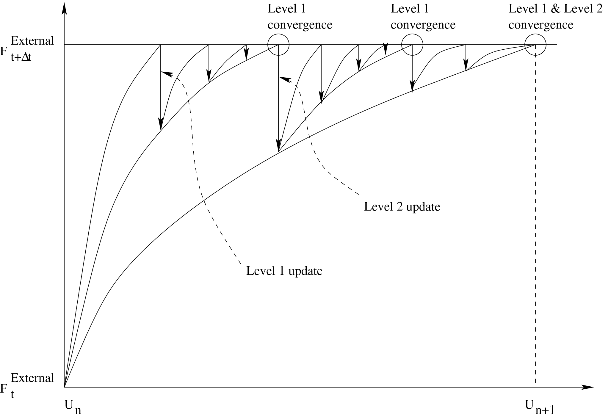
Fig. 4.1 Reaching convergence with controls and the multilevel solver.

Sierra/SM has four types of controls that can be used within the multilevel solver: control contact, control stiffness, control failure, and control damped solve.

Control contact is used to keep the set of nodes in contact constant during the solution of a model problem. Contact searches are performed during the multilevel solver updates. Control contact must be used for all problems that include a contact definition block, with the one exception of kinematic tied contact. If no control contact block is defined for problems that require one, a default control contact will be used. Control contact is not required for models that have only kinematic constraints, such as kinematic tied contact and MPCs. Control contact is documented in detail in Section 4.5.

Control stiffness is used to improve the conditioning of models that contain widely varying stiffness in different modes of material response. Such differences naturally exist for models with nearly incompressible materials where the bulk behavior is much stiffer than the shear behavior, for models with orthotropic and/or anisotropic materials that have much higher stiffness in preferred material directions, and for models containing several materials that are vastly different in their overall stiffness. Control stiffness works by scaling a given material response up (stiffening) or down (softening) to create a set of better conditioned model problems. For nearly incompressible materials, for instance, the bulk stress increments may be softened and/or the shear stress increments may be stiffened. For oriented materials, the stress increments in certain material directions are softened to create a material response that is more isotropic in nature. Finally, for the case where a material is much stiffer than the surrounding materials, both the bulk and shear stress increments are softened to create a response that has a stiffness much closer to that of the adjacent materials. Ultimately, as the control stiffness model problems progress, the true material response is recovered by building up stresses that correspond to the true material response. Special material models are required to use this capability, and Sierra/SM provides a number of material models that are designed to work with this capability. Control stiffness is documented in detail in Section 4.6.

Control failure is used to improve the conditioning of models that involve element death due to failure defined within a material model or to keep a consistent state for other failure criteria. Control failure used with material criterion element death limits the failure only to the single most critical element during each control failure iteration. Iterations of control failure continue until no additional elements are marked for failure. Control failure is documented in detail in Section 4.7.

Control damped solve is used on problems that have initial rigid body modes or other problems that are inherently difficult to solve with a quasistatic implicit solver alone. Some examples of problems that may benefit from this control are problems that require contact to be seated before preload, implicit contact problems where rebound or bounce occur, difficult implicit contact problems in general, and problems with softening materials. Control damped solve is documented in detail in Section 4.8.

The following is the basic structure of the SOLVER command block:

BEGIN SOLVER

  # CG solver commands:

  BEGIN CG
    # ... see Section 4.2, Section 4.3, and Section 4.4
  END [CG]

  # Multilevel control commands:

  BEGIN CONTROL CONTACT [<string>contact_name]
    # ... see Section 4.5
  END [CONTROL CONTACT <string>contact_name]

  BEGIN CONTROL STIFFNESS [<string>stiffness_name]
    # ... see Section 4.6
  END [CONTROL STIFFNESS <string>stiffness_name]

  BEGIN CONTROL FAILURE [<string>failure_name]
    # ... see Section 4.7
  END [CONTROL FAILURE <string>failure_name]

  BEGIN CONTROL DAMPED SOLVE [<string>ds_name]
    # ... see Section 4.8
  END [CONTROL DAMPED SOLVE <string>ds_name]

  # Predictor commands:

  BEGIN LOADSTEP PREDICTOR
    # ... see Section 4.9.1
  END [LOADSTEP PREDICTOR]

  LEVEL 1 PREDICTOR = <string>NONE|DEFAULT(DEFAULT)
  # see Section 4.9.2

END [SOLVER]

The SOLVER command block contains all solver-related commands, and must be present in the ADAGIO REGION command block. It is used regardless of whether the CG solver should be used alone or as a core solver in the multilevel solver. The CG command block (described in Section 4.2) is required for all models. If no multilevel controls are desired, the commands related to those controls are omitted from the SOLVER block.

In addition to the CG command block, the SOLVER command block contains command blocks that describe the controls used.

Aside from the command blocks for the core solver and the controls, the SOLVER block contains the LOADSTEP PREDICTOR command block, which is described in Section Section 4.9.1, and the LEVEL 1 PREDICTOR command line, which is described in Section 4.9.2.

Convergence tolerances for the CONTROL CONTACT, CONTROL STIFFNESS, and CONTROL DAMPED SOLVE solver levels are set within those command blocks while the tolerance of the core CG solver is set within the CG command block. Rather than using a convergence tolerance, the CONTROL FAILURE block is considered converged when no new elements are marked for failure during an iteration or when the maximum iterations is reached.

The commands within the CG command block are used in the same way whether the multilevel solver is used. It is, however, important to consider the role of tolerances within the multilevel solver. The convergence of the problem is controlled by the convergence of the highest solver level. For the multilevel solver to converge well, it is important for the core solver (or lower level of the solver, in the case of multiple levels) to reduce the residual by a certain amount during each model problem solution. For this reason, it is recommended that the solution tolerances be set an order of magnitude tighter for each lower level solver. The MINIMUM RESIDUAL IMPROVEMENT command in the CG command block is helpful for ensuring that the residual is reduced by the core solver during model problems, even though the residual might already be within the convergence tolerances (see Section 4.2.1).

4.1.1. Common Multilevel Solver Commands for All Controls

BEGIN SOLVER

  # CG solver commands:

  BEGIN CG

    # Parameters for CG
    # ... see :numref:`implicit-cg`, :numref:`implicit-ftprecon`, and :numref:`implicit-feti`

    # Diagnostic output commands, off by default:

    ITERATION PLOT = <integer>iter_plot
      [DURING <string list>period_names]
    ITERATION PLOT OUTPUT BLOCKS  = <string list>plot_blocks

  END [CG]

  #General Control commands:

  BEGIN CONTROL CONTACT|STIFFNESS|FAILURE|\{DAMPED SOLVE\} \textbackslash\#
    [<string>control_name]

    # ... see :numref:`implicit-contact`, :numref:`implicit-stiffness`, :numref:`implicit-failure`, and :numref:`implicit-damped`

    # Level selection command:

    LEVEL = <integer>control_level

    # Diagnostic output commands, off by default:

    ITERATION PLOT = <integer>iter_plot
      [DURING <string list>period_names]
    ITERATION PLOT OUTPUT BLOCKS  = <string list>plot_blocks

  END [CONTROL CONTACT|STIFFNESS|FAILURE|\{DAMPED SOLVE\} \textbackslash\#
    [<string>control_name]]

END [SOLVER]

Displayed in this section are common commands to all controls that can be used for the multilevel solver. Other commands may be used for specific controls, but those commands are not listed in this section. For commands specific to CONTROL CONTACT, see section Section 4.5. For commands specific to CONTROL STIFFNESS, see Section 4.6. For commands specific to CONTROL FAILURE, see Section 4.7. For commands specific to CONTROL DAMPED SOLVE, see Section 4.8.

LEVEL = <integer>control_level(1)

The LEVEL command line specifies the level in the multilevel solver at which contact, stiffness, and/or failure is controlled. The level parameter can have a value of either 1 or 2, with 1 being the default for all controls.

This command is used when multiple controls (e.g., control contact and control stiffness) are active in the multilevel solver. It is permissible for multiple controls to exist at a given level. In order to have a control at level 2, another control at level 1 is required. If control failure is defined, it should be the only control at the outermost (highest numerical value) level.

ITERATION PLOT = <integer>iter_plot
  [DURING <string list>period_names]
ITERATION PLOT OUTPUT BLOCKS  = <string list>plot_blocks

The iteration plot command lines can be used to output diagnostic information for each of the controls. The ITERATION PLOT command line allows plots of the current state of the model to be written to the output database during the control updates at a frequency specified by the value of iter_plot. The plots are output with fictitious time steps bounded by the step limits. Every time such a plot is generated, a message is sent to the log file. By default no iteration plots are generated. This feature is useful for debugging but should be used with care to avoid excessive output.

The output produced by iteration plots is sent by default to every active results output file specified by a RESULTS OUTPUT command block. The ITERATION PLOT OUTPUT BLOCKS command line can optionally be used to supply a list of output command block names to which iteration plots should be written. Each of the output block names listed in plot_blocks must match the name of a RESULTS OUTPUT command block (see Section 9.3.1). The ITERATION PLOT OUTPUT BLOCKS command line can be useful for directing iteration plots to separate output files so that these plots are separated from the converged solution output. It can also be used to send output plots for different levels of the multilevel solver to different files.