4.5. Control Contact

The multilevel solution control scheme used for contact is called control contact. Control contact alleviates some of the challenges associated with the nonlinear effects of contact by incrementally enforcing the contact nonlinearity outside the core solver. The specific steps taken during a control contact iteration depends on whether augmented Lagrange or kinematic enforcement is being used. Generally, the interactions (node-face or face-face pairs) that are being enforced are only changed once at the start of each control contact iteration and then held fixed during the core CG solve.

For Augmented Lagrange contact, see Section 4.5.2 for a detailed description.

The command block for control contact is:

BEGIN CONTROL CONTACT
  #
  # Convergence commands
  TARGET RESIDUAL = <real>target_resid
    [DURING <string list>period_names]
  TARGET RELATIVE RESIDUAL = <real>target_rel_resid(1.0e-3)
    [DURING <string list>period_names]
  TARGET RELATIVE CONTACT RESIDUAL =
    <real>target_rel_cont_resid
    [DURING <string list>period_names]
  ACCEPTABLE RESIDUAL = <real>accept_resid
    [DURING <string list>period_names]
  ACCEPTABLE RELATIVE RESIDUAL = <real>accept_rel_resid(1.0e-2)
    [DURING <string list>period_names]
  ACCEPTABLE RELATIVE CONTACT RESIDUAL =
    <real>accept_rel_cont_resid(1.0e-1)
    [DURING <string list>period_names]
  MINIMUM ITERATIONS  = <integer>min_iter(0)
    [DURING <string list>period_names]
  MAXIMUM ITERATIONS  = <integer>max_iter(100)
    [DURING <string list>period_names]
  #
  # level selection command
  LEVEL = <integer>control_contact_level(1)
  #
  # Augmented Lagrange enforcement commands used with
  # enforcement = al defined in the contact definition
  #
  # Gap Enforcement Options
  LAGRANGE ACCEPTABLE RELATIVE GAP = <real>(0.90)
    [DURING <string list>period_names]
  LAGRANGE ACCEPTABLE GAP = <real>(-1)
    [DURING <string list>period_names]
  #
  # Adaptive Penalty Options
  LAGRANGE INITIALIZE = NONE|MULTIPLIER|PENALTY|BOTH(MULTIPLIER)
    [DURING <string list>period_names]
  LAGRANGE ADAPTIVE PENALTY = OFF|SEPARATE|UNIFORM(OFF)
    [DURING <string list>period_names]
  LAGRANGE ADAPTIVE PENALTY GROWTH FACTOR = <real>(1.5)
    [DURING <string list>period_names]
  LAGRANGE ADAPTIVE PENALTY REDUCTION FACTOR = <real>(2.0/3.0)
    [DURING <string list>period_names]
  LAGRANGE ADAPTIVE PENALTY THRESHOLD = <real>(0.25)
    [DURING <string list>period_names]
  LAGRANGE MAXIMUM PENALTY MULTIPLIER = <real>(100.0)
    [DURING <string list>period_names]
  LAGRANGE MULTIPLIER PREDICTION SCALE FACTOR =<real>(0.85)
    [DURING <string list>period_names]
  #
  # Lagrange Tolerance Options
  LAGRANGE TOLERANCE = <real>(0.0)
    [DURING <string list>period_names]
  #
  # Miscellaneous Options
  LAGRANGE MAXIMUM UPDATES = <integer>(infinity)
    [DURING <string list>period_names]
  LAGRANGE NODAL STIFFNESS MULTIPLIER = <real>(0.0)
    [DURING <string list>period_names]
  #
  # Line search commands
  MAXIMUM LINE SEARCH STEP = <real>(2.0)
    [DURING <string list>period_names]
  MINIMUM LINE SEARCH STEP = <real>(0.01)
    [DURING <string list>period_names]
  #
  # Diagnostic output commands, off by default.
  ITERATION PLOT = <integer>iter_plot
    [DURING <string list>period_names]
  ITERATION PLOT OUTPUT BLOCKS = <string list>plot_blocks
END [CONTROL CONTACT]

For a problem containing a contact definition, control contact will be created by default if not defined in the input file. The default control contact will attempt to solve to a relative residual tolerance of \(1.0e^{-3}\) and will exist at level 1 of the solver. If non-default or advanced options are desired the control contact block must be defined directly.

4.5.1. Control Contact Commands

The line commands within the CONTROL CONTACT command block are used to control convergence during the contact updates, select the level for the contact control within the multilevel solver, and output diagnostic information. These commands are described in detail in sections Section 4.5.1.1 and Section 4.1.1.

4.5.1.1. Convergence Commands

The command lines listed in this section specify convergence criteria for the contact updates.

TARGET RESIDUAL = <real>target_resid
  [DURING <string list>period_names]
TARGET RELATIVE RESIDUAL =
  <real>target_rel_resid(1.0e-3)
  [DURING <string list>period_names]
TARGET RELATIVE CONTACT RESIDUAL = <real>target_rel_cont_resid(1.0e-3)
  [DURING <string list>period_names]
ACCEPTABLE RESIDUAL = <real>accept_resid
  [DURING <string list>period_names]
ACCEPTABLE RELATIVE RESIDUAL = <real>accept_rel_resid(1.0e-2)
  [DURING <string list>period_names]
ACCEPTABLE RELATIVE CONTACT RESIDUAL =
  <real>accept_rel_cont_resid(1.0e-1)
  [DURING <string list>period_names]
MINIMUM ITERATIONS = <integer>min_iter(0)
  [DURING <string list>period_names]
MAXIMUM ITERATIONS = <integer>max_iter(100)
  [DURING <string list>period_names]

Solver convergence is monitored for control contact in the same way as for the core CG solver. With the exception of two additional command lines used for controlling the residual due to contact, these command lines are the same as those for the core CG solver (described in Section 4.2.1). Here, however, these command lines are applied to the contact control level.

Contact convergence is evaluated by computing the \(L^2\) norm of the residual forces and comparing that with a target convergence criteria specified by the user in the control contact block. The relative residual is computed by dividing the residual by a reference quantity that is indicative of the current loading conditions on the model. Note the residual has units of force (or energy) while the relative residual is a dimensionless quantity where one or larger is an unconverged solution and the value moves towards zero for increasingly exact convergence.

The TARGET RESIDUAL command specifies the target convergence residual in terms of the actual residual norm. The TARGET RELATIVE RESIDUAL command specifies a convergence criterion in terms of the relative residual. If both command lines are specified, the multilevel solver will accept the contact solution as converged if either the target residual or the target relative residual is below the specified values.

The TARGET RELATIVE CONTACT RESIDUAL command line specifies a relative residual tolerance for just the nodes in contact. When this command is used this criterion must be satisfied in addition to the target residual or relative residual for all nodes. The default value for the target relative contact residual is the same value as the target relative residual or 10 times the target residual if the target relative residual has not been specified. As the contact residual is the residual on the subset of nodes of the model currently in contact the contact residual will always be strictly lower than the standard residual. For the TARGET RELATIVE CONTACT RESIDUAL to have any effect the value must be set below the TARGET RELATIVE RESIDUAL. A small TARGET RELATIVE CONTACT RESIDUAL command can be used to give improved confidence in the accuracy of the solution in the contact zone.

Acceptable convergence criteria can also be used for contact convergence. If the solution has not converged to the specified target before the maximum number of iterations is reached, the residual is checked against the acceptable convergence criteria. These criteria are specified via the ACCEPTABLE RESIDUAL, ACCEPTABLE RELATIVE RESIDUAL, and ACCEPTABLE RELATIVE CONTACT RESIDUAL command lines. The concepts of acceptable residual, relative residual, and relative contact residual are the same as those used for the targets. If the solution has not met the target criteria but has met the acceptable criteria, the solution is allowed to proceed. The defaults for each of these acceptable criteria are 10 times the corresponding target criteria defaults.

Control contact will use the same reference type (EXTERNAL, BELYTSCHKO, ENERGY, etc.) as the underlying CG solver block.

The MAXIMUM ITERATIONS and MINIMUM ITERATIONS command lines specify the maximum and minimum number of contact updates, respectively. The default minimum number of iterations, min_iter, is 0. If a number greater than 0 is specified, the multilevel solver will update contact at least that many times, regardless of whether the convergence criteria have been met.

For an explanation of commands common to all controls, see Section 4.1.1.

4.5.1.2. Tips on Setting Control Contact and CG tolerances

Generally the target residual in the CG block should be set to about an order of magnitude below the target residual in the CONTACT block, while the acceptable residual in the CG block should be set to a very large number. The acceptable should be large enough to assure solution acceptance for any remotely reasonable result.

For each control contact step, a set of active contact constraints is held fixed. The core CG solver subsequently solves the analysis problem subject to a linearized version of those active contact constraints. Occasionally control contact will pick a set of constraints that cannot be solved; for example, creating two constraints that conflict such that the solution is over determined. When this happens, the CG solver will never be able to drop the residual of the over-constrained system. In this case, contact needs to try again to pick a better constraint set. When CG hits the maximum number of iterations and meets the high acceptable tolerance, it will return to the contact solver. Though the residual is still high, it usually has enough information to at least help contact select an improved constraint set. Note, when using control contact the actual true tolerance of the solution is the control contact residual. The CG residual is used for the intermediate model problems. Thus, if control contact eventually converges to a reasonably small residual, the solution itself is correct even if some of the intermediate CG steps only converged on a high acceptable residual.

4.5.1.3. Augmented Lagrange Gap Enforcement Options

# Gap Enforcement Options
LAGRANGE ACCEPTABLE RELATIVE GAP = <real>(0.90)
  [DURING <string list>period_names]
LAGRANGE ACCEPTABLE GAP = <real>(-1)
  [DURING <string list>period_names]

The LAGRANGE ACCEPTABLE RELATIVE GAP and LAGRANGE ACCEPTABLE GAP can be used to ensure that the penetration or gap is sufficiently removed before moving on to the next loadstep. Augmented Lagrange enforcement applies equal and opposite forces with each control contact iteration. These options force contact iterations to continue until both residual balance and a sufficient amount of penetration or gap is removed.

The LAGRANGE ACCEPTABLE RELATIVE GAP by default is set to 0.90. The control contact solver level will continue iterating until the largest contact relative gap value is less than or equal to the specified value. The relative gap is the gap value divided by the respective interaction tolerance and is unitless. Failing to converge contact to a relative gap below 1.0 risks missing contact on the subsequent loadstep.

The LAGRANGE ACCEPTABLE GAP by default is not specified. The control contact solver level will keep iterating until the largest contact gap value is less than or equal to the specified value. The gap value specified is the actual largest gap value and has the units of length. This command is most appropriately used when model dimensions are well understood, manual normal tolerances have been set, and a known gap tolerance is desired.

4.5.1.4. Augmented Lagrange Initialization Commands

LAGRANGE INITIALIZE = NONE|MULTIPLIER|PENALTY|BOTH(MULTIPLIER)
  [DURING <string list>period_names]

The LAGRANGE INITIALIZE command is used to control how Lagrange multipliers are set at the beginning of a load step. The default value of MULTIPLIER specifies that the Lagrange multipliers will be initialized to some factor of the previous step Lagrange multipliers. By default this multiplication factor is 0.85 and can be changed with the LAGRANGE MULTIPLIER PREDICTION SCALE FACTOR command.

The NONE option turns off initialization of the Lagrange multipliers, setting them to zero. This option may aid convergence in some very nonlinear analyses where the next load step is in a completely different contact state than the previous load step. The PENALTY option initializes Lagrange multipliers based off of material stiffness and gap. The BOTH initializes Lagrange multipliers based off of both the old multiplier and the material stiffness and gap in an attempt to achieve a more efficient prediction. It is generally recommended that only the MULTIPLIER or NONE options be used as the penalty based initialization is experimental at this time.

4.5.1.5. Augmented Lagrange Adaptive Penalty Commands

# Adaptive Penalty Options
LAGRANGE ADAPTIVE PENALTY = OFF|SEPARATE|UNIFORM(OFF)
  [DURING <string list>period_names]
LAGRANGE ADAPTIVE PENALTY GROWTH FACTOR = <real>(1.5)
  [DURING <string list>period_names]
LAGRANGE ADAPTIVE PENALTY REDUCTION FACTOR = <real>(2.0/3.0)
  [DURING <string list>period_names]
LAGRANGE ADAPTIVE PENALTY THRESHOLD = <real>(0.25)
  [DURING <string list>period_names]
LAGRANGE MAXIMUM PENALTY MULTIPLIER = <real>(100.0)
  [DURING <string list>period_names]
LAGRANGE MULTIPLIER PREDICTION SCALE FACTOR =<real>(0.85)
  [DURING <string list>period_names]

The command lines listed above can be used to control the augmented Lagrange contact adaptive penalty algorithm. Augmented Lagrange contact enforcement is activated when ENFORCEMENT = AL is set in the contact definition block.

The LAGRANGE ADAPTIVE PENALTY command indicates how the penalty multiplier will be adjusted as the problem progresses. The option SEPARATE scales the penalty differently for each contact interaction. The option UNIFORM scales all interactions equally. The default option is OFF.

The LAGRANGE ADAPTIVE PENALTY GROWTH FACTOR command sets the adaptive penalty growth factor, while the LAGRANGE ADAPTIVE PENALTY REDUCTION FACTOR command sets the adaptive penalty reduction factor. The LAGRANGE ADAPTIVE PENALTY THRESHOLD sets the adaptive penalty threshold. The LAGRANGE MAXIMUM PENALTY MULTIPLIER sets the maximum penalty multiplier, which is the upper bound on the penalty multiplier when running augmented Lagrange contact.

In augmented Lagrange contact, if the current gap magnitude is greater than the previous gap magnitude, the penalty multiplier is reduced by multiplying it by the penalty reduction factor. If the current gap magnitude is between the previous gap magnitude and the previous gap magnitude times the penalty threshold, the penalty multiplier is increased by multiplying it by the penalty growth factor. The lower bound for the penalty multiplier is 1.0 and the upper bound is the maximum penalty multiplier.

The LAGRANGE MULTIPLIER PREDICTION SCALE FACTOR sets a scaling factor on the Lagrange multipliers when moving from one load step to the next. Generally the converged Lagrange multipliers at a new load step will be close to the multipliers obtained in the previous load step. When predicting the next configuration, a default scaling factor of 0.85 is applied to the previous Lagrange multipliers to reduce the danger of overshooting the contact solution. A value closer to 1.0 may accelerate convergence but may also introduce issues by overshooting the true contact solution.

4.5.1.6. Augmented Lagrange Tolerance

# Tolerance Options
LAGRANGE TOLERANCE = <real>(0.0)
  [DURING <string list>period_names]

The LAGRANGE TOLERANCE can be used to set the Lagrange multiplier tolerance for updating. Once the change to the Lagrange multiplier is less than the tolerance, the Lagrange multiplier will no longer be updated. The default is 0.0, which always updates the Lagrange multiplier.

4.5.1.7. Augmented Lagrange Miscellaneous Options

# Miscellaneous Options
LAGRANGE MAXIMUM UPDATES = <integer>(infinity)
  [DURING <string list>period_names]
  [DURING <string list>period_names]
LAGRANGE NODAL STIFFNESS MULTIPLIER = <real>(0.0)
  [DURING <string list>period_names]

The LAGRANGE MAXIMUM UPDATES command sets the maximum number of augmented Lagrange updates performed during a load step. By default, the Lagrange multiplier is always updated. Setting this to zero makes contact a pure penalty formulation.

The LAGRANGE NODAL STIFFNESS MULTIPLIER sets a scale factor on the amount of contact stiffness included in the nodal preconditioner. The default value is 0.0, which means no contact stiffness is present in the nodal preconditioner. A value of 1.0 distributes the full contact stiffness to the contact nodes and a value much greater than 1.0 effectively pins (or fixes) the contact nodes in the nodal preconditioner.

4.5.2. Augmented Lagrange Control Contact

For augmented Lagrange enforcement, a search is only performed once in the predicted configuration of a new load step. It is crucial that the predicted configuration be reasonable. Experience has shown that no prediction is often best, so it is recommended that the load step predictor be turned off when using augmented Lagrange enforcement for contact. This can be accomplished by setting the scale factor predictor to zero (see Section 4.9.1).

The contact search provides a set of all possible interactions. In the log file example in Section 4.5.2.1, the listed NUM INTERACTIONS is the number of possible interactions that were found in the contact search. Each interaction is a node-face or face-face pair, depending on the constraint formulations used in the contact definition.

Interactions can exist in one of three states: RELEASED, CAPTURED, or DUBIOUS. Tied interactions are determined once during the search and can only be CAPTURED or RELEASED. Other interactions start in a DUBIOUS or RELEASED state after the search. To reduce chatter, these interactions can only move to CAPTURED or RELEASED by moving through the DUBIOUS state.

The DUBIOUS state serves as an intermediate state. During a model problem, interactions in the DUBIOUS state are enforced with a nonlinear penalty kernel during the model problem, while interactions in the CAPTURED state use a linear penalty kernel. This is why the first model problem is often the most difficult. The logic to move interactions between states is based on the gapping history combined with the value of the accumulated Lagrange multiplier.

During a contact update, the Lagrange multiplier is augmented before the state determination by adding the penalty kernel to the Lagrange multiplier. This update causes an additional residual imbalance from what was solved for in the model problem. If this update is sufficiently small, you will converge at the control contact level and will not return to level 0 to solve the residual imbalance. The maximum relative change in the value of the Lagrange multiplier is listed in the log file as RELATIVE LMULT CHANGE. Because the convergence is determined exclusively on the residual balance, it is sometimes desirable to set a LAGRANGE TOLERANCE so that if the change in the Lagrange multiplier is small enough, the update is not done. This preserves the residual balance determined in the model problem, assuming there is no change in the interaction states.

As contact iterations progress, the values of MAX GAP, MAX RELATIVE GAP and RELATIVE LMULT CHANGE should decrease and the set of interactions should stop changing (signified by the output line NO ACTIVE SET CHANGE). Successive iterations should report a RELATIVE RESIDUAL for control contact closer to the RELATIVE RESIDUAL reported in the model problem until convergence is reached.

Many of the log file quantities described here are also stored as global variables (see Table 9.4).

4.5.2.1. Augmented Lagrange Control Contact Log File Example

===========================================================================================================
Begin load step =    37 Solution period Adagio_Procedure_time_control_1 is  14.8% complete
        Old Time       Time Step        New Time       Stop Time     CPU Time(s)    Wall Time(s)
      7.4000e-03      2.0000e-04      7.6000e-03      5.0000e-02      3.8784e+00      4.0469e+00
-----------------------------------------------------------------------------------------------------------
                                         MP                  RELATIVE     EXTERNAL
                                       ITER     RESIDUAL     RESIDUAL    REFERENCE      ENERGY DISPLACEMENT
-----------------------------------------------------------------------------------------------------------
                                          0    9.358e-03    6.885e-02    1.359e-01           -            -
                                         16    1.814e-06    1.595e-05<T  1.137e-01   4.634e-17    8.057e-08
-----------------------------------------------------------------------------------------------------------
MAX GAP               = 2.779e-05 PREVIOUS = 0.000e+00
MAX RELATIVE GAP      = 6.175e-03 PREVIOUS = 0.000e+00
NUM INTERACTIONS      = 60
RELEASED INTERACTIONS = 0
CAPTURED INTERACTIONS = 60
DUBIOUS INTERACTIONS  = 0
RELATIVE LMULT CHANGE = 1.465e-01
ACTIVE SET CHANGE
-----------------------------------------------------------------------------------------------------------
CONTACT ITERATION =            0
ABSOLUTE RESIDUAL =    3.444e-03
RELATIVE RESIDUAL =    2.914e-02
-----------------------------------------------------------------------------------------------------------
. ( Skipped Contact Iteration 1 - 9 for readability ) ...
-----------------------------------------------------------------------------------------------------------
                                         MP                  RELATIVE     EXTERNAL
                                       ITER     RESIDUAL     RESIDUAL    REFERENCE      ENERGY DISPLACEMENT
-----------------------------------------------------------------------------------------------------------
                                          0    8.104e-05    6.810e-04    1.190e-01           -            -
                                          5    1.295e-06    1.088e-05<T  1.190e-01   9.540e-19    2.180e-08
-----------------------------------------------------------------------------------------------------------
MAX GAP               = 1.136e-06 PREVIOUS = 1.129e-06
MAX RELATIVE GAP      = 1.514e-04 PREVIOUS = 1.506e-04
NUM INTERACTIONS      = 60
RELEASED INTERACTIONS = 4
CAPTURED INTERACTIONS = 56
DUBIOUS INTERACTIONS  = 0
RELATIVE LMULT CHANGE = 7.380e-03
NO ACTIVE SET CHANGE
-----------------------------------------------------------------------------------------------------------
CONTACT ITERATION =           10
ABSOLUTE RESIDUAL =    5.179e-05
RELATIVE RESIDUAL =    4.352e-04<T
----------------------------------------------------------------------------------
   LEVEL 1                                                  ITERATIONS          TOTAL
   CONTACT     MODEL PROB      LOAD STEP        AVERAGE          TOTAL         CPU(s)
 CONVERGED             11            114             10           4069      4.825e+00

4.5.3. Kinematic Control Contact

For kinematic enforcement, a search is performed each contact iteration to provide a set of nodes in contact. This constraint set is held constant during the subsequent model problem. For frictional contact, side B nodes are fixed to side A faces during the CG iterations. For frictionless contact, the side B nodes are fixed in the normal direction but are allowed to slide during the CG iterations. After model problem convergence, the constraint set is updated to reflect the changing contact conditions. This update gives rise to a force imbalance to be solved in another model problem.

Changing or updating the constraint set is called a contact update. Multiple contact updates are typically required before equilibrium is achieved. The contact update includes a search, a gap removal, an equilibrium query, and a slip calculation if equilibrium is not satisfied.

New constraints are detected in the search phase based on the current deformed configuration of the model. If a node is found to penetrate a side A surface, the node is added to the set of constraints.

The gap removal phase involves creating or destroying constraints and calculating push-back vectors for side B nodes. A penetration may be removed at once (the default behavior), or it may be incrementally removed over a number of model problems. For interactions where contacting surfaces are free to separate, a side B node constraint continues to exist as long as there is a compressive force between the side B node and the side A surface. The constraint changes during the gap removal phase to reflect changes in the shape and orientation of the side A surface. Constraints are destroyed when a tensile force exceeding a specified tolerance (see Section 8.6.2.11) exists at the contact interface.

During the slip portion of the contact update, a residual force is calculated at each node and resolved into normal and tangential components. This force reflects changes in residual due to gap removal that occurred earlier in the update. For frictional contact, the friction coefficient is used to determine the tangential load capacity. If the tangential loads exceed this capacity, nodes will slip.

The procedure for kinematic control contact is illustrated in the following sequence of figures. It is assumed in these figures that control contact is the level 1 solver, so the model problems are directly solved by the core solver. In Fig. 4.2, the model problem has three constraints that are enforced during iterations of the core solver. However, during solution of the model problem an additional node penetrates the side A surface.

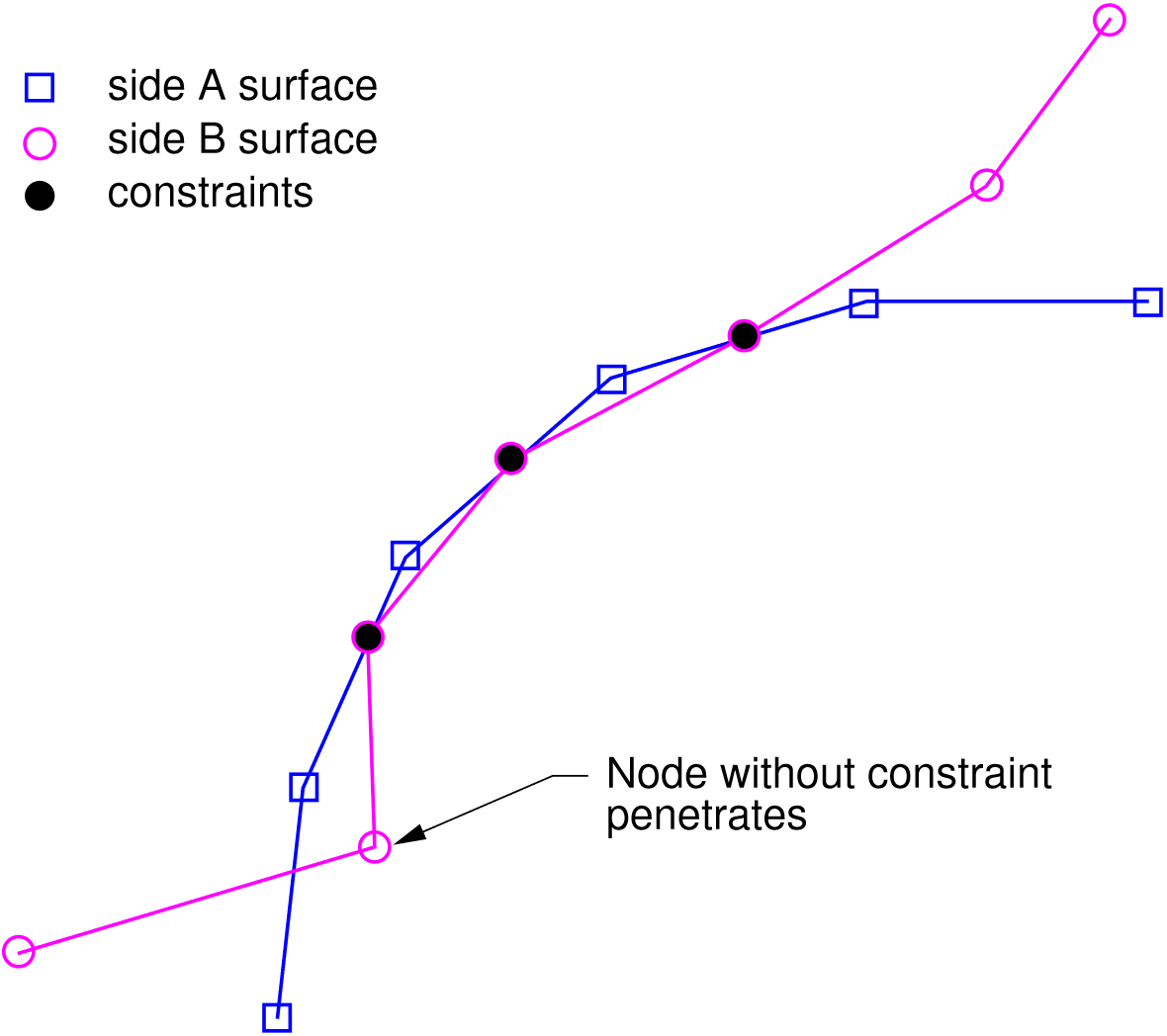
Fig. 4.2 Contact configuration at the beginning of the contact update.

Once the model problem has converged, a contact update is performed. During the search, one node if found to have penetrated the surface, resulting in a new constraint for this node. A push-back vector is calculated for this node to remove the penetration. In the gap removal portion of the update (Fig. 4.3), one of the constraints is found to have accumulated a tensile force large enough that surfaces should separate, indicating that this constraint should be eliminated.

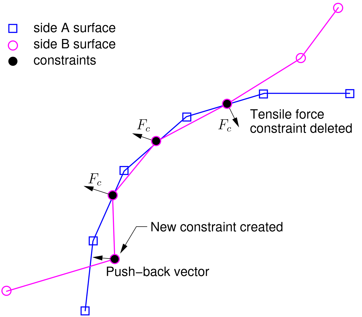
Fig. 4.3 Contact gap removal (after contact search).

In the second phase of the contact update, slip is allowed to occur along the contact interface. After the gaps are removed, the external and internal force vectors are recomputed, and forces are partitioned along normal and tangential directions of the side A surface. This process is illustrated in Fig. 4.4.

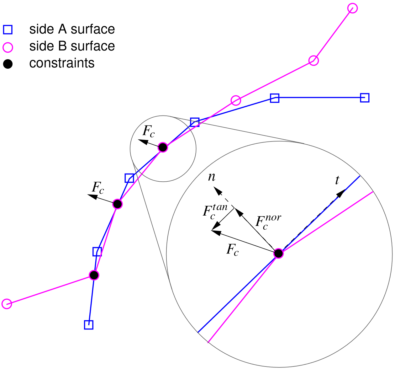
Fig. 4.4 Contact slip calculations.

4.5.4. CG with Control Contact Input Example

begin solver
  begin control contact
    target relative residual = 1.0e-4
    maximum iterations       = 100
  end
  begin cg
    acceptable relative residual = 1.0e+10
    target relative residual = 1.0e-6
    maximum iterations       = 100
    iteration print          = 25
    begin full tangent preconditioner
      minimum smoothing iterations = 25
    end
  end
end