7. Stress Measures

7.1. Cauchy Stress

In this chapter we discuss the quantification of force intensity, or stress, within a body undergoing potentially large amounts of deformation. We begin with the Cauchy stress tensor \(\mathbf{T}\) and note that, provided we associate this object with the spatial configuration, this object can be interpreted exactly as in the infinitesimal case outlined in Section 2. In the current notational framework, we interpret the components of \(\mathbf{T}\), denoted as \(T_{ij}\), which represent forces per unit areas in the spatial configuration at a given spatial point \(\mathbf{x} \in \varphi_t (\Omega)\).

It will be necessary in our description to consider related measures of stress defined in terms the reference and rotated configurations. To motivate this discussion, we reconsider the concept of traction discussed previously in the context of the infinitesimal elastic system. Recall that given a plane passing through the point of interest \(\mathbf{x}\), the traction, or force per unit area acting on this plane, is given by the formula

(7.1)\[t_i = T_{ij} n_j ,\]

where \(n_j\) is the unit normal vector to the plane in question.

7.2. Nanson’s Formula

We consider two differential vectors, \(\mathrm{d}\mathbf{r}_1\) and \(\mathrm{d}\mathbf{r}_2\), as illustrated in Fig. 7.1. We assume that \(\mathrm{d}\mathbf{r}_1\) and \(\mathrm{d}\mathbf{r}_2\) are linearly independent and that both have spatial point \(\mathbf{x}\) as their base point. We further assume that their orientations are such that the following relation from basic geometry holds:

(7.2)\[\mathrm{d}\mathbf{r}_1 \times \mathrm{d}\mathbf{r}_2 = \mathbf{n} \mathrm{d}a,\]

where \(\mathrm{d}a\) is the (differential) area of the parallelogram encompassed by \(\mathrm{d}\mathbf{r}_1\) and \(\mathrm{d}\mathbf{r}_2\).

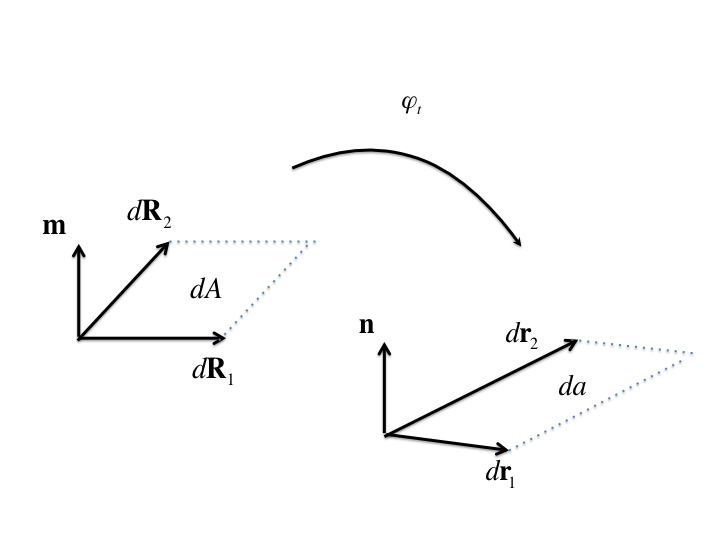
Fig. 7.1 Notation for derivation of Nanson’s formula.

As discussed in Section 5 (see (5.5)), we can think of the differential vectors \(\mathrm{d} \mathbf{r}_1\) and \(\mathrm{d} \mathbf{r}_2\) as the current positions of reference differential vectors \(\mathrm{d} \mathbf{R}_1\) and \(\mathrm{d} \mathbf{R}_2\), which are based at \(\mathbf{X}=\varphi^{-1}_t (\mathbf{x})\). In index notation, we can relate these two sets of differential vectors using the deformation gradient via

(7.3)\[(\mathrm{d}\mathbf{r}_1)_i = F_{iI} (\mathrm{d}\mathbf{R}_1)_I ,\]

and

(7.4)\[(\mathrm{d}\mathbf{r}_2)_i = F_{iI} (\mathrm{d}\mathbf{R}_2)_I .\]

We now seek to re-express (7.2) in terms of reference quantities. Working in index notation, we write

(7.5)\[\begin{split}\begin{aligned} n_i \mathrm{d}a & = e_{ijk} F_{jJ} (\mathrm{d}\mathbf{R}_1)_J F_{kK} (\mathrm{d}\mathbf{R}_2)_K \\ & = e_{ljk} \delta_{li} F_{jJ} (\mathrm{d}\mathbf{R}_1)_J F_{kK} (\mathrm{d}\mathbf{R}_2)_K \\ & = e_{ljk} F_{lL} F^{-1}_{Li} F_{jJ} (\mathrm{d}\mathbf{R}_1)_J F_{kK} (\mathrm{d}\mathbf{R}_2)_K \end{aligned}\end{split}\]

We extract and manipulate a particular product in the last line of (7.5), namely \(e_{ljk} F_{lL} F_{jJ} F_{kK}\). One can show by a case-by-case examination that the following relation holds:

(7.6)\[e_{ljk} F_{lL} F_{jJ} F_{kK} = e_{LJK} e_{ljk} F_{l1} F_{j2} F_{k3} .\]

Recall from Section 5, (5.10) that \(J=\text{ det}(\mathbf{F})\) has the following representation in index notation:

(7.7)\[J = \text{ det}(\mathbf{F}) = e_{ljk} F_{l1} F_{j2} F_{k3}\]

Combination of (7.5), (7.6), and (7.7) yields the following result:

(7.8)\[\begin{split}\begin{aligned} n_i \mathrm{d}a & = J e_{LJK} F^{-1}_{Li} (\mathrm{d}\mathbf{R}_1)_J (\mathrm{d}\mathbf{R}_2)_K \\ & = J F^{-1}_{Li} m_L \mathrm{d}A. \end{aligned}\end{split}\]

In (7.8), \(\mathrm{d}A\) is the differential reference area spanned by \(\mathrm{d}\mathbf{R}_1\) and \(\mathrm{d}\mathbf{R}_2\), and \(\mathbf{m}\) is the reference unit normal to this area.

In direct notation, we express this result as

(7.9)\[\mathbf{n}\mathrm{d}a = J \mathbf{F}^{-T} \mathbf{m} \mathrm{d}A .\]

(7.9) is referred to as Nanson’s formula and it is important, among other reasons, because it provides the appropriate change-of-variables formula for surface integrals in the reference and current configurations.

7.3. First and Second Piola-Kirchhoff Stress

We want to compute a differential force, which is the product of the traction acting on our plane at \(\mathbf{x}\) and the differential area under consideration. Denoting this differential force by \(\mathrm{d}\mathbf{f}\), we write

(7.10)\[\mathrm{d}\mathbf{f} = \mathbf{t}\mathrm{d}a = \mathbf{T}\mathbf{n}\mathrm{d}a = J \mathbf{T}\mathbf{F}^{-T} \mathbf{m} \mathrm{d} A .\]

In examining (7.10), we find that the following definition is useful:

(7.11)\[\mathbf{P}(\mathbf{X}) = J(\mathbf{X}) \mathbf{T} \left( \varphi_t(\mathbf{X}) \right) \mathbf{F}^{-T} \left( \varphi_t(\mathbf{X}) \right) .\]

This allows us to write

(7.12)\[\mathrm{d}\mathbf{f} = \mathbf{P} \mathbf{m} \mathrm{d}A .\]

In (7.12), the product \(\mathbf{P}\mathbf{m}\) represents a traction, the current force, \(\mathrm{d}\mathbf{f}\), divided by the reference area, \(\mathrm{d}A\). The tensor \(\mathbf{P}\) is called the (First) Piola-Kirchhoff Stress and \(\mathbf{P}\mathbf{m}\) is called the Piola Traction. Similar to the Piola Traction, the First Piola-Kirchhoff Stress measures stress in terms of forces in the current configuration and areas in the reference configuration. The one-dimensional manifestation of this stress measure is the engineering stress, \(\sigma_E\), originally defined in (1.3).

It is worthy to note that \(\mathbf{P}\) is neither a pure spatial nor a pure reference object. A reference object for stress can be constructed by performing a pull-back of the spatial Cauchy stress tensor \(\mathbf{T}\) to the reference configuration:

(7.13)\[\begin{split}\begin{array} {l l} \mathbf{S}( \mathbf{X} ) & = J \mathbf{F}^{-1} \left( \varphi_t (\mathbf{X}) \right) \mathbf{T} \left( \varphi_t (\mathbf{X}) \right) \mathbf{F}^{-T} \left( \varphi_t (\mathbf{X}) \right) \\ {} & = \mathbf{F}^{-1} \left( \varphi_t (\mathbf{X}) \right) \mathbf{P} (\mathbf{X}) . \end{array}\end{split}\]

\(\mathbf{S}\) is called the Second Piola-Kirchhoff Stress and it is purely a reference object. We note, in particular, that \(\mathbf{S}\) is a symmetric tensor, while \(\mathbf{P}\) is not symmetric in general.

This same concept of pull-back can be employed to define a stress tensor in the rotated configuration, which we shall denote as \(\pmb{\mathit{T}}\). This rotated tensor is defined as

(7.14)\[\pmb{\mathit{T}} = \mathbf{R}^{T} \left( \varphi_t (\mathbf{X}) \right) \mathbf{T} \left( \varphi_t (\mathbf{X}) \right) \mathbf{R} \left( \varphi_t (\mathbf{X}) \right) .\]

As was the case with the rotated configuration quantities introduced in Section 6, this definition will be of particular importance in the later examination of frame indifference.