8. Balance Laws

In this chapter, we examine the local forms of the various conservation laws as expressed in the various reference frames we have introduced (spatial, reference, and rotated). To expedite our development, we first discuss how integral representations of balances can be converted to point wise conservation principles, a process known as localization.

8.1. Localization

Suppose we consider an arbitrary volume of material in the reference configuration, \(V \subset \Omega\), of a solid body as depicted in Fig. 8.1. Suppose further that we can establish the following generic integral relation over this volume:

(8.1)\[\int_V f(\mathbf{X}) \mathrm{d}V = 0,\]

where \(f\) is some reference function, be it scalar-, vector-, or tensor-valued, defined over all of \(\Omega\). If (8.1) holds true for each and every subvolume \(V\) of \(\Omega\), then the localization theorem states that

(8.2)\[f = 0 \text{ pointwise in } \Omega.\]

The interested reader should consult reference [[1]] for elaboration on this principle.

It should be noted that the same procedure can be applied spatially. In other words, if we are working with a spatial object, we might consider arbitrary volumes \(v\) in the spatial domain, and if the following holds for a spatial object \(g\) for all \(v\):

(8.3)\[\int_v g(\mathbf{x}) \mathrm{d}v = 0,\]

then \(g(\mathbf{x}) = 0\) throughout \(\varphi_t(\Omega)\).

Our primary interest in these localization principles will be to take the well known conservation laws for control volumes and convert them to their local counterparts valid point wise throughout the domain.

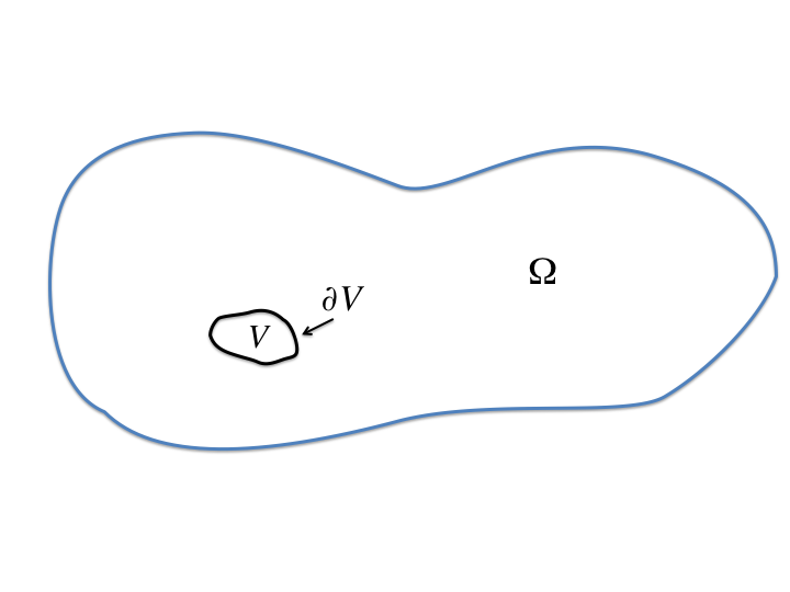
Fig. 8.1 Notation for the localization concept.

8.2. Conservation of Mass

For conservation of mass, we consider a fixed control volume, \(v\), in the spatial domain, completely filled with our solid body at the instant in question as the body moves through it. We can write a conservation of mass for this control volume via

(8.4)\[-\int_{\partial v} \rho \mathbf{v} \cdot \mathbf{n} \mathrm{d}a = \int_v \frac{\partial \rho}{\partial t} \mathrm{d}v ,\]

where the left-hand side can be interpreted as the net mass influx to the control volume, and the right-hand side is the rate of mass accumulation inside the control volume. Applying the divergence theorem to the left-hand side gives

(8.5)\[-\int_{v} \nabla \cdot \left( \rho \mathbf{v} \right) \mathrm{d}v = \int_v \frac{\partial \rho}{\partial t} \mathrm{d}v .\]

This can be further rearranged to yield

(8.6)\[\int_{v} \left( \frac{\partial \rho}{\partial t} + \nabla \rho \cdot \mathbf{v} + \rho (\nabla \cdot \mathbf{v}) \right) \mathrm{d}v = 0 ,\]

which can be established for any arbitrary spatial volume \(v\). Applying the localization theorem gives the local expression of continuity, which may be familiar to those versed in fluid mechanics:

(8.7)\[\frac{\partial \rho}{\partial t} + \nabla \rho \cdot \mathbf{v} + \rho (\nabla \cdot \mathbf{v}) = \dot{\rho} + \rho(\nabla \cdot \mathbf{v}) = 0,\]

where the concept of the material time derivative has been employed (cf. (6.5)).

A reference configuration representation of continuity is desirable for the study of solid mechanics. Therefore we convert (8.6) to a reference configuration integral to obtain:

(8.8)\[\int_{V=\varphi^{-1}_t (v)} ( \dot{\rho} + \rho \dot{\mathbf{F}}:\mathbf{F}^{-T} ) J \mathrm{d}V = 0,\]

where the transformation between \(\mathrm{d}v\) and \(\mathrm{d}V\) is accomplished using (5.9) and the chain rule is used to convert \(\nabla \cdot \mathbf{v}\) via

(8.9)\[\begin{split}\begin{aligned} v_{i,i}(\mathbf{x}) & = \frac{\partial}{\partial x_i} V_i \left(\varphi^{-1}_t(\mathbf{x}) \right) \\ & = \frac{\partial}{\partial X_I} V_i \left(\varphi^{-1}_t(\mathbf{x}) \right) \frac{\partial X_I}{\partial x_i} \left(\varphi^{-1}_t(\mathbf{x}) \right) \\ & = \dot{F_{iI}} \left(\varphi^{-1}_t(\mathbf{x}) \right) F^{-1}_{Ii}\left(\varphi^{-1}_t(\mathbf{x}) \right) , \end{aligned}\end{split}\]

which is the index notation form of \(\dot{\mathbf{F}}:\mathbf{F}^{-T}\). Applying the localization theorem in the reference configuration gives

(8.10)\[\dot{\rho} J + \rho J \dot{\mathbf{F}}:\mathbf{F}^{-T} = 0 ,\]

which holds point wise in \(\Omega\).

Working in index notation, we can further simplify (8.10) by concentrating on the term \(J\dot{\mathbf{F}}:\mathbf{F}^{-T}\). We compute the material time derivative of \(J\) as

(8.11)\[\dot{J} = \frac{\partial J}{\partial F_{mM}} \dot{F_{mM}} ,\]

where

(8.12)\[\begin{split}\begin{aligned} \frac{\partial J}{\partial F_{mM}} & = \frac{\partial}{\partial F_{mM}} (e_{ijk} F_{i1} F_{j2} F_{k3}) \\ & = e_{ijk} \delta_{im} \delta_{M1} F_{j2} F_{k3} + e_{ijk} \delta_{jm} \delta_{M2} F_{i1} F_{k3} + e_{ijk} \delta_{km} \delta_{M3} F_{i1} F_{j2} \\ & = e_{ijk} F_{iN} F^{-1}_{Nm} \delta_{M1} F_{j2} F_{k3} + e_{ijk} F_{jN} F^{-1}_{Nm} \delta_{M2} F_{i1} F_{k3} + e_{ijk} F_{kN} F^{-1}_{Nm} \delta_{M3} F_{i1} F_{j2} , \end{aligned}\end{split}\]

which simplifies to

(8.13)\[\begin{split}\begin{aligned} \frac{\partial J}{\partial F_{mM}} & = J F^{-1}_{1m} \delta_{M1} + J F^{-1}_{2m} \delta_{M2} + J F^{-1}_{3m} \delta_{M3} \\ & = J F^{-1}_{Im} \delta_{MI} = J F^{-1}_{Mm} . \end{aligned}\end{split}\]

Substitution of (8.13) into (8.11) gives

(8.14)\[\dot{J} = J F^{-1}_{Mm} \dot{F_{mM}} ,\]

which is the index notation form of

(8.15)\[\dot{J} = J \mathbf{F^{-1}} : \dot{\mathbf{F}} .\]

Finally, substitution of (8.15) into (8.10) gives

(8.16)\[\dot{\rho}J + \rho \dot{J} = \frac{\mathrm{d}}{\mathrm{d}t} (\rho J) = 0 .\]

(8.16) is the reference configuration version of the continuity equation, which tells us that the product of the density and deformation gradient determinant must be invariant with time for all material points. This is commonly enforced in practice by assigning a reference density \(\rho_0\) to all material points. If the current density \(\rho\) is computed via

(8.17)\[\rho = \frac{1}{J} \rho_0 ,\]

then (8.16) is automatically satisfied (recall that the Jacobian is unity in the reference configuration).

8.3. Conservation of Linear Momentum

Considering once more a fixed control volume \(v\), the control volume balance of linear momentum can be expressed as

(8.18)\[\int_{\partial v} (\rho \mathbf{v}) \mathbf{v} \cdot \mathbf{n} \mathrm{d}a + \int_{v} \frac{\partial}{\partial t} (\rho \mathbf{v}) \mathrm{d}v = \int_{v} \mathbf{f} \mathrm{d}v + \int_{\partial v} \mathbf{t} \mathrm{d}a .\]

On the left-hand side, the first term expresses the momentum out flux and the second term represents the rate of accumulation inside the control volume. This net change of momentum is produced by the total resultant force on the system, i.e., the right-hand side of the equation, which is equal to the sum effect of the body forces \(\mathbf{f}\) and the surface tractions \(\mathbf{t}\).

Applying the divergence theorem to both surface integrals, we find that

(8.19)\[\int_{\partial v} (\rho \mathbf{v}) \mathbf{v} \cdot \mathbf{n} \mathrm{d}a = \int_{v} \left[\nabla \cdot (\rho \mathbf{v})\mathbf{v} + \rho (\nabla \mathbf{v}) \mathbf{v} \right] \mathrm{d}v ,\]

and

(8.20)\[\int_{\partial v} \mathbf{t} \mathrm{d}a = \int_{\partial v} \mathbf{T} \mathbf{n} \mathrm{d}a = \int_{v} \nabla \cdot \mathbf{T} \mathrm{d}v.\]

Substituting (8.19) and (8.20) into (8.18), and rearranging, gives

(8.21)\[\int_{v} \left[ \nabla \cdot \mathbf{T} + \mathbf{f} - \rho \frac{\partial \mathbf{v}}{\partial t} - \rho(\nabla \mathbf{v}) \mathbf{v} - \frac{\partial \rho}{\partial t} \mathbf{v} - (\nabla \rho \cdot \mathbf{v})\mathbf{v} - \rho(\nabla \cdot \mathbf{v})\mathbf{v} \right] \mathrm{d}v = 0.\]

Employing the spatial form of the continuity (8.6) and recalling the formula for the material time derivative (6.5) gives

(8.22)\[\int_{v} \left[ \nabla \cdot \mathbf{T} + \mathbf{f} - \rho \dot{\mathbf{v}} \right] \mathrm{d}v = 0.\]

The localization theorem then implies

(8.23)\[\nabla \cdot \mathbf{T} + \mathbf{f} = \rho \dot{\mathbf{v}}\]

point wise, which is recognized as the same statement of linear momentum balance utilized in our earlier treatment of linear elasticity, (2.2).

In large deformation problems it is desirable to also have a reference configuration form of (8.23). Converting (8.22) to its index form, we have

(8.24)\[\int_{v} \left[ T_{ij,j} + f_i - \rho \dot{v}_i \right] \mathrm{d}v = 0.\]

Working with the stress divergence term first, we write

(8.25)\[T_{ij,j} = \frac{\partial T_{ij}}{\partial X_J} \frac{\partial X_J}{\partial x_j} = \frac{\partial T_{ij}}{\partial X_J} F^{-1}_{Jj}.\]

Using (7.11), we can write

(8.26)\[\frac{\partial T_{ij}}{\partial X_J} = \frac{\partial}{\partial X_j} \left( \frac{1}{J} P_{iI} F_{jI} \right) = \frac{-1}{J^2} \frac{\partial J}{\partial F_{kK}} \frac{\partial F_{kK}}{\partial X_{j}} P_{iI} F_{jI} + \frac{1}{J} \frac{\partial}{\partial X_J} (P_{iI} F_{jI}).\]

Now using (8.13), we can simplify (8.26) and post multiply \(F^{-1}_{Jj}\) to obtain:

(8.27)\[\frac{\partial T_{ij}}{\partial X_J} F^{-1}_{Jj} = \frac{-1}{J} F^{-1}_{Kk} \frac{\partial F_{kK}}{\partial X_J} P_{iJ} + \frac{1}{J} \frac{\partial P_{iI}}{\partial X_I} + \frac{1}{J} F^{-1}_{Jj} \frac{\partial F_{jI}}{\partial X_J} P_{iI}\]

The first and last terms on the right-hand side of (8.27) cancel each other due to the fact that \(\frac{\partial F_{jI}}{\partial X_J} = \frac{\partial F_{jJ}}{\partial X_I}\). Therefore we have

(8.28)\[\frac{\partial T_{ij}}{\partial X_J} F^{-1}_{Jj} = \frac{1}{J} \frac{\partial P_{iI}}{\partial X_I} .\]

Combining this result with (8.25) and (8.24), and applying a change of variables, gives

(8.29)\[\int_V (P_{iI,I} + b_i -\rho_0 \dot{V}_i ) \mathrm{d}V = 0 ,\]

where \(b_i = J f_i\), the prescribed body force per unit reference volume. Employing the localization theorem gives

(8.30)\[\nabla_0 \cdot \mathbf{P} + \mathbf{b} = \rho_0 \dot{V}\]

point wise in \(\Omega\), which expresses the balance of linear momentum in terms of reference coordinates. In (8.30), \(\nabla_0\) is the gradient operator with respect to the reference configuration.

8.4. Conservation of Angular Momentum

Again considering an arbitrary control volume in the spatial frame, we write its balance of angular momentum via

(8.31)\[\int_{\partial v} (\mathbf{x} \times \rho \mathbf{v}) \mathbf{v} \cdot \mathbf{n} \mathrm{d}a + \int_{v} \frac{\partial}{\partial t} (\mathbf{x} \times \rho \mathbf{v} ) \mathrm{d}v = \int_{v} (\mathbf{x} \times \mathbf{f})\mathrm{d}v + \int_{\partial v} \mathbf{x} \times \mathbf{t} \mathrm{d}a ,\]

where the terms on the left-hand side are the out flux and accumulations terms, and the terms on the right-hand side represent the total resultant torque.

Working this time in index notation, we apply the divergence theorem to the surface integrals as follows:

(8.32)\[\int_{\partial v} e_{ijk} \rho x_j v_k v_l n_l \mathrm{d}a = \text{ } \int_v \left( \rho_{,l} e_{ijk} x_j v_k v_l + e_{ijk} \rho \delta_{jl} v_k v_l + e_{ijk} \rho x_j v_{k,l} v_l + e_{ijk} \rho x_j v_k v_{l,l} \right) \mathrm{d}v ,\]

and

(8.33)\[\int_{\partial v} e_{ijk} x_j T_{kl} n_l \mathrm{d}a = \int_v \left( e_{ijk} x_j T_{kl,l} + e_{ijk} T_{kj} \right) \mathrm{d} v .\]

Substituting (8.32) and (8.33) into (8.31), and rearranging terms, reveals that

(8.34)\[\begin{split}\begin{aligned} \int_{v} \Bigg( e_{ijk} x_j \left( T_{kl,l} + f_k - \rho \frac{\partial v_k}{\partial t} - \rho \frac{\partial v_k}{\partial x_l} v_l \right) \\ - e_{ijk} x_j v_k \left( \frac{\partial \rho}{\partial t} + \frac{\partial \rho}{\partial x_l} v_l + \rho v_{l,l} \right) \\ + e_{ijk} T_{kl} - \rho e_{ijk} \rho v_j v_k \Bigg) \mathrm{d}v = 0 . \end{aligned}\end{split}\]

Using (8.24) and (8.7), and noting that the cross product of a vector with itself is zero, we can simplify (8.34) and apply the localization theorem to conclude

(8.35)\[e_{ijk} T_{kl} = 0 ,\]

which, in turn, implies the following three equations:

(8.36)\[T_{23} = T_{32} ,\: T_{13} = T_{31} ,\: T_{21} = T_{12} .\]

In other words, the symmetry of the Cauchy stress tensor is a direct consequence of the conservation of angular momentum. Use of (7.13) and (7.14), respectively, reveals that the Second Piola-Kirchhoff stress \(\mathbf{S}\) and the rotated stress tensor \(\pmb{\mathit{T}}\) are likewise symmetric. The First Piola-Kirchhoff stress is not symmetric and is not, in fact, a tensor in the purest sense because it does not fully live in either the spatial or reference frame.

8.5. Stress Power

We examine the consequences of a control volume expression of energy balance. We assume herein a purely mechanical description and, to begin, that there is no mechanical dissipation, so that the system we consider conserves energy exactly. In other words, all work put into the system through the applied loads goes either into stored internal elastic energy or into kinetic energy.

With this in mind, the conservation of energy for a spatial control volume is written as

(8.37)\[\int_{\partial v} \left( e + \frac{1}{2} \rho \mathbf{v} \cdot \mathbf{v} \right) \mathbf{v} \cdot \mathbf{n} \mathrm{d}a + \int_{v} \frac{\partial}{\partial t} \left( e + \frac{1}{2} \rho \mathbf{v} \cdot \mathbf{v} \right) \mathrm{d}v = \int_{v} \mathbf{f} \cdot \mathbf{v} \mathrm{d} v + \int_{\partial v} \mathbf{t} \cdot \mathbf{v} \mathrm{d}a ,\]

where \(e\) is the internal stored energy (i.e., elastic energy) per unit spatial volume.

As we have done previously, we apply the divergence theorem to the surface integrals:

(8.38)\[\begin{split}\begin{aligned} \int_{\partial v} \left( e + \frac{1}{2} \rho \mathbf{v} \cdot \mathbf{v} \right) \mathbf{v} \cdot \mathbf{n} \mathrm{d}a = \int_{v} & \Bigg[ \nabla \cdot \mathbf{v} \left( e + \frac{1}{2} \rho \mathbf{v} \cdot \mathbf{v} \right) + \nabla e \cdot \mathbf{v} \\ & + \frac{1}{2} \nabla \rho \cdot \mathbf{v}(\mathbf{v} \cdot \mathbf{v}) + \rho \mathbf{v} \cdot (\nabla \mathbf{v})\mathbf{v} \Bigg] \mathrm{d}v , \end{aligned}\end{split}\]

and

(8.39)\[\int_{\partial v} \mathbf{t} \cdot \mathbf{v} \mathrm{d}a = \int_{v} \left[ \mathbf{T}:\nabla \mathbf{v} + (\nabla \cdot \mathbf{T}) \cdot \mathbf{v} \right] \mathrm{d}v .\]

Substituting (8.38) and (8.39) into (8.37), and rearranging, gives

(8.40)\[\begin{split}\begin{aligned} 0 =\int_{v} & \left[ \left( \nabla \cdot \mathbf{T} + \mathbf{f} - \rho \frac{\partial \mathbf{v}}{\partial t} - \left(\rho \, \nabla \mathbf{v} \right) \mathbf{v} \right) \cdot \mathbf{v} \right. \\ {} & - \frac{1}{2} \mathbf{v} \cdot \mathbf{v} \left( \frac{\partial \rho}{\partial t} + (\nabla \cdot \mathbf{v}) \rho + \nabla \rho \cdot \mathbf{v} \right) \\ {} & \left. + \mathbf{T}: \nabla \mathbf{v} - (\nabla \cdot \mathbf{v}) e - \dot{e} \right] \mathrm{d}v . \end{aligned}\end{split}\]

Using (8.24) and (8.7), we find

(8.41)\[0 = \int_{v} \left[ \mathbf{T} : \nabla \mathbf{v} - (\nabla \cdot \mathbf{v}) e - \dot{e} \right] \mathrm{d}v .\]

Splitting (8.41) into two integrals, we have

(8.42)\[0 = \int_{v} \mathbf{T} : \nabla \mathbf{v} \mathrm{d}v - \int_{v} \left( (\nabla \cdot \mathbf{v})e + \dot{e} \right) \mathrm{d}v .\]

We now convert (8.42) to the reference configuration and apply localizations. In so doing, we recognize that the second integral in (8.42) can be treated directly analogous to that of (8.6), with the density \(\rho\) in (8.6) replaced by the energy \(e\) in the current case. The result of this manipulation will be analogous to (8.16) with \(e\) substituted for \(\rho\). In other words, we have

(8.43)\[\int_{v} \left( (\nabla \cdot \mathbf{v})e + \dot{e} \right) \mathrm{d}v = \int_{V} \frac{d}{dt} (e J) \mathrm{d}V .\]

Concentrating on the first integral and using (6.12) and (8.11) to aid in the calculation, we find

(8.44)\[\begin{split}\begin{aligned} \int_{v} \mathbf{T} : \nabla \mathbf{v} \mathrm{d}v & = \int_{V} (\mathbf{T} \circ \varphi^{-1}) : (\mathbf{L} \circ \varphi^{-1}) J \mathrm{d}V \\ {} & = \int_{V} (\mathbf{T} \circ \varphi^{-1}) : (\dot{\mathbf{F}} \mathbf{F}^{-1}) J \mathrm{d}V = \int_{V} \mathbf{P} : \dot{\mathbf{F}} \mathrm{d}V . \end{aligned}\end{split}\]

Plugging the results of (8.43) and (8.44) into (8.42) and employing the localization theorem, we determine that

(8.45)\[\frac{d}{dt} (e J) = \dot{E} = \mathbf{P}:\dot{\mathbf{F}}\]

point wise in \(\Omega\), where \(E\) is the stored elastic energy per unit reference volume. Therefore, \(\mathbf{P}:\dot{\mathbf{F}}\) represents the rate of energy input into the material by the stress (per unit volume), commonly known as the stress power. Taking into account the various measures of stress and deformation rate we have considered, it can be shown that for a given material point, the stress power can be written in the following alternative forms:

(8.46)\[\textbf{stress power} = \mathbf{P}:\dot{\mathbf{F}} = \frac{1}{2} \mathbf{S}\dot{\mathbf{C}} = J \mathbf{T}:\mathbf{D} = J \pmb{\mathit{T}}:\pmb{\mathit{D}} .\]

It should be noted that this definition can be used also for dissipative (i.e., non-conservative) materials but the interpretation changes. The stress power in that case is the sum of the rate of increase of stored energy and the rate of energy dissipated by the solid.

8.6. Thermodynamics

Finally we discuss the application of the laws of thermodynamics to large deformation Lagrangian mechanics. Recalling the notation from Section 4, we consider the first and second laws applied to a body \(\Omega\) in the reference (i.e., material) configuration.

First Law

The first law states that the change in internal energy, change in kinetic energy, external power, and heat flux over the body must be balanced:

\[\dot{ \mathcal{E} } + \dot {\mathcal{K}} = \mathcal{W} + \mathcal{Q}\]

where

• \(\mathcal{E}\), the total internal energy, is given by

  \[\mathcal{E} = \int_{\Omega} \rho_0 w \, dV,\]

  where \(w\) is the specific internal energy (both elastic and dissipated),

• \(\mathcal{K}\), the kinetic energy, is given by

  \[\mathcal{K} = \int_{\Omega} \frac{1}{2} \rho_0 \left| \mathbf{v} \right|^2 \, dV,\]

• \(\mathcal{W}\), the conventional external power, is given by

  \[\mathcal{W} = \int_{\partial \Omega} \mathbf{T}\mathbf{n} \cdot \mathbf{v} \, d\Gamma + \int_{\Omega} \mathbf{b} \, dV,\]

• \(\mathcal{Q}\), the heat flux, is given by

  \[\mathcal{Q} = -\int_{\partial \Omega} \mathbf{q} \cdot \mathbf{n} \, d\Gamma + \int_{\Omega} q \, dV,\]

  where \(q\) is the scalar heat supply, and \(\mathbf{q}\) is the heat flux vector.

The corresponding local energy balance can be readily derived by applying the divergence theorem and power balance on sub-regions:

(8.47)\[\rho_0 \dot{w} = \mathbf{T} : \mathbf{D} - \nabla_0 \cdot \mathbf{q} + q,\]

where \(\nabla_0 \cdot\) is the divergence operator in the reference configuration.

Second Law

The second law of thermodynamics states that the entropy of an isolated system can not decrease. The global inequality over \(\Omega\) corresponding to this statement is

\[\int_{\Omega} \rho_0 \dot{\eta} \, dV \geq -\int_{\partial \Omega} \frac{\mathbf{q}}{\theta} \, d\Gamma + \int_{\Omega} \frac{q}{\theta} \, dV,\]

where \(\eta\) is the specific entropy, \(\theta\) is the absolute temperature, \(\frac{\mathbf{q}}{\theta}\) is the entropy flux, and \(\frac{q}{\theta}\) is the entropy supply. The corresponding local entropy imbalance can be derived using the divergence theorem and localization to sub-regions:

\[\rho_0 \dot{\eta} \geq -\nabla_0 \cdot \left( \frac{\mathbf{q}}{\theta} \right) + \frac{q}{\theta}.\]

Using (8.47) and some manipulation this can be rewritten

(8.48)\[\mathbf{T} : \mathbf{D} - \rho_0 \, \left( \dot{e} + \eta \dot{\theta} \right) - \frac{1}{\theta} \mathbf{q} \cdot \nabla_0 \theta \geq 0,\]

where \(e\), the specific free-energy (i.e., the elastic energy), is given by

\[e = w - \theta \eta.\]

In the absence of thermal effects, (8.48) reduces to

\[\mathbf{T} : \mathbf{D} \geq \rho_0 \, \dot{e},\]

which states that the internal power expenditure (stress power) must exceed the rate of increase of stored energy. More simply put, the dissipated power in the body must always be positive.

The references for chapter 8 are [[1][2][3][4]].

---

[1] (1,2)

M.E. Gurtin. An Introduction to Continuum Mechanics. Mathematics in Science and Engineering. Academic Press, Inc., 1982.

[2]

Y.C. Fung. Foundations of Solid Mechanics. Prentice-Hall, Inc, 1965.

[3]

J.E. Marsden and T.J.R. Hughes. Mathematical Foundations of Elasticity. Dover, 1983.

[4]

M.E. Gurtin, E. Fried, and L. Anand. The Mechanics and Thermodynamics of Continua. Cambridge University Press, 2010.