5. Deformation Measures

5.1. Deformation Gradient

Furthering our discussion of large deformation solid mechanics, we continue to use the notation presented in Fig. 4.1. We restrict our attention to some time \(t \in (0,T)\), and consider the corresponding configuration mapping \(\varphi_t\), which can be mathematically represented via \(\varphi_t : \bar \Omega \rightarrow \mathbb{R}_3\). The deformation gradient \(\mathbf{F}\) is given by the gradient of this transformation,

(5.1)\[\mathbf{F} = \frac{\partial \varphi_t}{ \partial \mathbf{X}} ,\]

or in index notation,

(5.2)\[F_{iJ} = \frac{\partial \varphi_{ti}}{ \partial X_J} .\]

In (5.2) and throughout this documented unless otherwise noted, lower case indices are associated with coordinates in the spatial frame and upper case indices with material coordinates. Repeated indices of either case imply summation.

The deformation gradient is the most basic object used to quantify the local deformation at a point in a solid. Most kinematic measures and concepts we will discuss rely on it explicitly for their definition. For example, elementary calculus provides a physical interpretation of the determinant of \(\mathbf{F}\). Consider a cube of material in the reference configuration (see Fig. 5.1) whose sides are assumed to be aligned with the coordinate axes \(X_I, I=1,2,3\). The initial differential volume \(\mathrm{d} V\) of this cube is given by

(5.3)\[\mathrm{d} V = \mathrm{d} X_1 \mathrm{d} X_2 \mathrm{d} X_3 .\]

If we now consider the condition of this cube of material after the deformation \(\varphi_t\) is applied, we notice that its volume in the current configuration \(\mathrm{d} v\) is that of the parallelepiped spanned by the three vectors \(\varphi_t ( \overrightarrow{\mathrm{d}X_J})\), where the notation \(\overrightarrow{\mathrm{d}X_J}\) is used to indicate a reference vector in coordinate direction \(J\) with magnitude \(\mathrm{d} X_J\). This volume can be written in terms of the vector triple product,

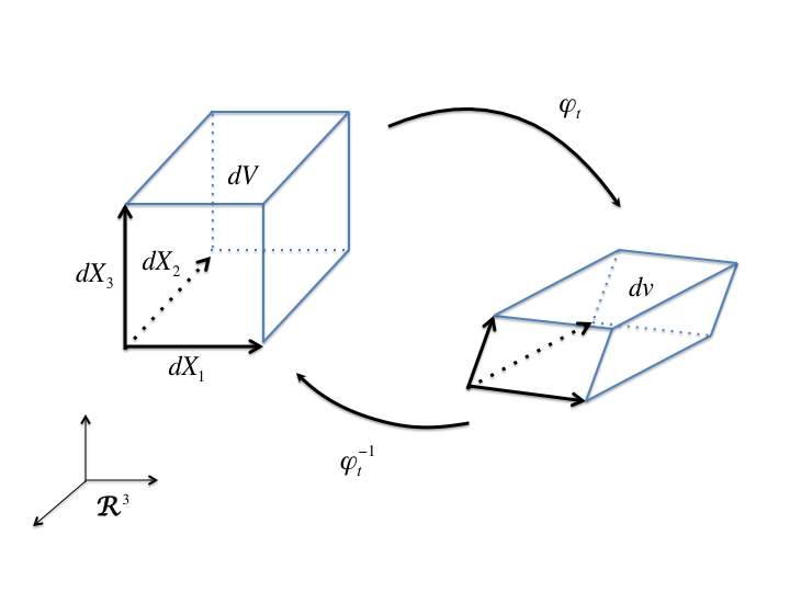
(5.4)\[\mathrm{d} v = \varphi_t ( \overrightarrow{\mathrm{d}X_1}) \cdot \varphi_t ( \overrightarrow{\mathrm{d}X_2}) \cdot \varphi_t ( \overrightarrow{\mathrm{d}X_3}) .\]

../_images/deformation_measures-fig01.png — Fig. 5.1 Deformation of a volume element as described by the configuration mapping \(\varphi_t\).

If we consider any differential vector \(\overrightarrow{\mathrm{d} R}\) in the reference configuration, the calculus of differentials tells us that application of the mapping \(\varphi_t\) will produce a differential vector \(\overrightarrow{\mathrm{d} r} = \varphi_t ( \overrightarrow{\mathrm{d} R} )\) whose coordinate are given by

(5.5)\[(\overrightarrow{\mathrm{d} r})_i = \frac{\partial \varphi_{ti}}{\partial X_K}( \overrightarrow{\mathrm{d} R} )_K .\]

Application of this logic to the particular differential vectors \(\overrightarrow{\mathrm{d} R_J}\) leads one to conclude that

(5.6)\[\begin{split}(\varphi_t (\overrightarrow{\mathrm{d} X_J}))_i = \begin{cases} F_{i1} \mathrm{d} X_1, \quad J=1, \\ F_{i2} \mathrm{d} X_2, \quad J=2, \\ F_{i3} \mathrm{d} X_3, \quad J=3. \\ \end{cases}\end{split}\]

We can write (5.4) in index notation by first noting that the cross product of two vectors \(\mathbf{a}\) and \(\mathbf{b}\) is written as

(5.7)\[(\mathbf{a} \times \mathbf{b})_i = \mathrm{e}_{ijk} a_j b_k,\]

where \(\mathrm{e}_{ijk}\), the permutation symbol, is defined as

(5.8)\[\begin{split}\mathrm{e}_{ijk} = \begin{cases} 1 & \mathrm{ if } \; (i,j,k) = (1,2,3) \; \mathrm{ or } \; (2,3,1) \; \mathrm{ or } \; (3,1,2), \\ -1 & \mathrm{ if } \; (i,j,k) = (3,2,1) \; \mathrm{ or } \; (2,1,3) \; \mathrm{ or } \; (1,3,2), \\ 0 & \mathrm{ otherwise} . \end{cases}\end{split}\]

(5.4) can then expressed as

\[\begin{split}\begin{aligned} \label{deformation_measure:eq:09} \mathrm{d}v & = F_{i1} \mathrm{d} X_1 (\mathrm{e}_{ijk} F_{j2} \mathrm{d} X_2 F_{k3} \mathrm{d} X_3) \\ {} & = \mathrm{e}_{ijk} F_{i1} F_{j2} F_{k3} \mathrm{d} X_1 \mathrm{d} X_2 \mathrm{d} X_3 \\ {} & = \det (\mathbf{F}) \mathrm{d} V , \end{aligned}\end{split}\]

where we have used (5.3) and the fact that \(\det (\mathbf{F}) = \mathrm{e}_{ijk} F_{i1} F_{j2} F_{k3}\) (which can be verified through trial). Introducing the notation \(J=\det (\mathbf{F})\), we conclude

(5.9)\[\mathrm{d}v = J \mathrm{d} V .\]

(5.9) tells us that the deformation \(\varphi_t\) converts reference differential volumes \(\mathrm{d}V\) to current volumes \(\mathrm{d}v\) according to the determinant of the deformation gradient. For this mapping to make physical sense, the current volume \(\mathrm{d}v\) should be positive which then places a physical restriction upon the deformation gradient \(\mathbf{F}\) that must be obeyed point wise throughout the domain,

(5.10)\[J = \det (\mathbf{F}) = \det \left( \frac{\partial \varphi}{\partial \mathbf{X}} \right) > 0 .\]

This physical restriction has important mathematical consequences as well. According to the inverse function theorem of multivariate calculus, a smooth function whose gradient has a nonzero determinant possesses a smooth and differentiable inverse. Since we have assumed \(\varphi_t\) to be smooth and physical restrictions demand that \(J>0\), we can conclude that a function \(\varphi_t^{-1}\) exists and is differentiable; in fact, the gradient of this function is given by

(5.11)\[\frac{\partial \varphi_t^{-1}}{\partial \mathbf{X}} = \mathbf{F}^{-1}.\]

We will assume throughout the remainder of our discussion that \(J>0\), so that such an inverse is guaranteed to exist.

5.2. Polar Decomposition

With the definition of \(\mathbf{F}\) in hand, we turn our attention to the quantification of local deformation in a body. For any matrix such as \(\mathbf{F}\), whose determinant is positive, the following decomposition can always be made:

(5.12)\[\mathbf{F} = \mathbf{R} \mathbf{U} = \mathbf{V} \mathbf{R}.\]

In (5.12), \(\mathbf{R}\) is a proper orthogonal tensor (right-handed rotation), while \(\mathbf{U}\) and \(\mathbf{V}\) are positive-definite, symmetric tensors. One can show that under the conditions stated, the decompositions in (5.12) can always be made and that they are unique. The interested reader should consult Reference [[1]] of Chapter 1 for details. The decompositions \(\mathbf{RU}\) and \(\mathbf{VR}\) in (5.12) are called right and left polar decompositions of \(\mathbf{F}\), respectively. \(\mathbf{R}\) is often called the rotation tensor, while \(\mathbf{U}\) and \(\mathbf{V}\) are sometimes referred to as the right and left stretches.

The significance of the polar decomposition is made more clear in Fig. 5.2, where we consider the deformation of a neighborhood of material surrounding a point \(\mathbf{X} \in \Omega\). (5.5) shows that the full deformation gradient maps arbitrary reference differentials into their current positions at time \(t\). By considering the polar decomposition, we see that the deformation of material neighborhoods of infinitesimal extent can always be conceptualized in two ways. In the right polar decomposition, \(\mathbf{U}\) contains all information necessary to describe the distortion of a neighborhood of material, while \(\mathbf{R}\) then maps this distorted neighborhood into the current configuration through pure (right-handed) rotation. On the other hand, in the left polar decomposition, the rotation \(\mathbf{R}\) is considered first followed by the distortion \(\mathbf{V}\). In developing measures of local deformation, we can thus focus on either \(\mathbf{U}\) or \(\mathbf{V}\). The choice of which decomposition to use is typically based on the coordinates in which we wish to write the strains. The right stretch \(\mathbf{U}\) most naturally takes reference coordinates as arguments, while the left stretch \(\mathbf{V}\) is ordinarily written in terms of spatial coordinates. This can be expressed as

(5.13)\[\mathbf{F}(\mathbf{X}) = \mathbf{R}(\mathbf{X}) \mathbf{U}(\mathbf{X}) = \mathbf{V}(\varphi(\mathbf{X})) \mathbf{R}(\mathbf{X}).\]

In characterizing large deformations, it is also convenient to define the right and left Cauchy-Green tensors via

(5.14)\[\mathbf{C} = \mathbf{F}^T\mathbf{F}\]

and

(5.15)\[\mathbf{B} = \mathbf{F}\mathbf{F}^T .\]

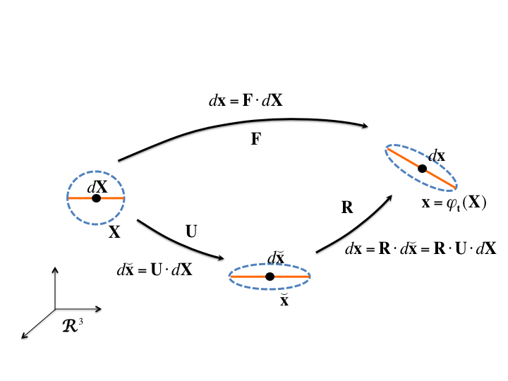
../_images/deformation_measures-fig02.png — Fig. 5.2 Dotted outline indicates infinitesimal neighborhood of point \(X\).)

The right Cauchy-Green tensor is ordinarily considered to be a material object \(\mathbf{C}(\mathbf{X})\), while the left Cauchy-Green tensor is a spatial object \(\mathbf{B}(\varphi_t (\mathbf{X}))\). Since \(\mathbf{R}\) is orthogonal, one can write

(5.16)\[\mathbf{R}^T\mathbf{R} = \mathbf{R}\mathbf{R}^T = \mathbf{I},\]

where \(\mathbf{I}\) is the \(3 \times 3\) identity tensor. Manipulating (5.13) through (5.15) reveals that

(5.17)\[\mathbf{U} = \mathbf{C}^{\frac{1}{2}}\]

and

(5.18)\[\mathbf{V} = \mathbf{B}^{\frac{1}{2}}.\]

One can see the connection with small strain theory by considering the Green strain tensor \(\mathbf{E}\) defined with respect to the reference configuration,

(5.19)\[\mathbf{E} = \frac{1}{2} (\mathbf{C}-\mathbf{I}).\]

We define the reference configuration displacement field \(\mathbf{u}\), such that

(5.20)\[\mathbf{u}(\mathbf{X}) = \varphi(\mathbf{X}) - \mathbf{X}.\]

Working in index notation, we write \(\mathbf{E}\) in terms of \(\mathbf{u}\)

(5.21)\[\begin{split}\begin{aligned} E_{IJ} & = \frac{1}{2}(C_{IJ}-\delta_{IJ}) = \frac{1}{2} \left( F_{iI}F_{iJ}-\delta_{IJ} \right) \\ {} & = \frac{1}{2} \left( \frac{\partial}{\partial X_I}(u_i+X_i) \frac{\partial}{\partial X_J}(u_i+X_i)- \delta_{IJ} \right) \\ {} & = \frac{1}{2} \left( \left(\frac{\partial u_i}{\partial X_I} + \delta_{iI} \right) \left(\frac{\partial u_i}{\partial X_J} + \delta_{iJ} \right) - \delta_{IJ} \right) \\ {} & = \frac{1}{2} \left( \delta_{iI} \frac{\partial}{\partial X_J}(u_i) + \delta_{iJ} \frac{\partial}{\partial X_I} (u_i) + \frac{\partial u_i}{\partial X_I} \frac{\partial u_j}{\partial X_J} \right) \end{aligned}\end{split}\]

In the case where the displacement gradients are small, i.e., \(| \frac{\partial U_i}{\partial X_J} | \ll 1\), the quadratic term in (5.21) will be much smaller that the terms linear in the displacement gradients. If, in addition, the displacement components \(u_i\) are very small when compared with the size of the body, then the distinction between reference and spatial coordinates becomes unnecessary and (5.21) simplifies to

(5.22)\[E_{IJ} \approx \frac{1}{2} \left( \frac{\partial u_I}{\partial X_J} +\frac{\partial u_J}{\partial X_I} \right) ,\]

which is identical to the infinitesimal case (cf. (2.5)).

The references for Chapter 5 are [[2][1][3]].