4.34. Wire Mesh Model

4.34.1. Theory

The wire mesh model was developed at Sandia National Laboratories for use with layered sequences of metallic wire meshes and cloth fabric. Model development was based on an extensive series of experiments performed on these materials (see [[1]]) and used an existing model for rigid polyurethane foams as a starting point [[2]].

To be able to analyze the response of this material, the Cauchy stress tensor is first decomposed into its principal components, \(\sigma^i\). Each principal stress is evaluated independently and two behaviors are considered depending on whether or not the material is in tension or compression. Under a tensile load, the material is taken to be perfectly plastic above a yield stress, \(\tau\). For compressive loads, it is assumed that the materials hardens functionally with the volumetric engineering strain, \(\varepsilon_{\text{V}}\). In this formulation, an arbitrary form of this hardening function, \(\bar{\sigma}\left(\varepsilon_{\text{V}}\right)\) is assumed although in the original work [[1]],

(4.177)\[\bar{\sigma}\left(\varepsilon_{\text{V}}\right) = a e^{-b\varepsilon_{\text{V}}},\]

with \(a\) and \(b\) as material constants, was used.

With these assumptions, the yield function of the \(i^{\text{th}}\) principal stress, \(f^i\), may be written as,

\[\begin{split}f^i = \left\{\begin{array}{cc} \sigma^i-\tau, & \sigma^i \geq 0 \\ -\sigma^i-\bar{\sigma}\left(\varepsilon_{\text{V}}\right) & \sigma^i < 0 \end{array}\right. .\end{split}\]

where \(\tau\) is the isotropic tensile strength of the material.

Similar to the rigid polyurethane foam model [[1]], the flow rule is defined as:

\[d^{\text{p}}_{ij} = \dot{\gamma}^{1}P^{1}_{ijkl} \sigma_{kl} + \dot{\gamma}^{2}P_{ijkl}^{2}\sigma_{kl} + \dot{\gamma}^{3}P^{3}_{ijkl}\sigma_{kl}\]

with \(\dot{\gamma}^{i}\) being the magnitude of the \(i^{\text{th}}\) plastic strain increment and \(P^{r}_{ijkl}\) is the fourth-order principal projection operator defined as,

\[P^{r}_{ijkl} = n^{r}_i n^{r}_j n^{r}_k n^r_l\]

in which \(n^{r}_i\) is the corresponding direction vector of principal stress, \(\sigma^r\). With this definition,

\[\sigma^r=\sigma_{ij}P^r_{ijkl}\sigma_{kl}.\]

4.34.2. Implementation

The wire mesh model is implemented in a hypoelastic fashion similar to the previous elastic-plastic models. First, a trial (unrotated) stress is calculated assuming a purely elastic deformation increment,

\[T^{tr}_{ij}=T^n_{ij}+\Delta t\left(\lambda\delta_{ij}d_{kk}+2\mu d_{ij}\right).\]

Corresponding principal stresses and their complementary directions are then found using the robust, analytical algorithm put forth in [[3]]. The principal stresses are denoted \(\sigma^{r}\) and their eigenvectors are symbolically represented by \(\hat{e}^{r}_{i}\). Here, \(r=~1,~2,\) or \(3\) refer to the respective eigenvalue/vector pair and are not summed unless explicitly indicated. Before evaluating the respective yield functions, the current volumetric engineering strain, \(\varepsilon_{\text{V}}^{n+1}\), must be determined. To this end, the current strain tensor, \(\varepsilon_{ij}\), is determined via,

\[\varepsilon^{n+1}_{ij}=\varepsilon^n_{ij}+\Delta td_{ij},\]

and the volumetric engineering strain is,

\[\varepsilon_{\text{V}}^{n+1}=\exp{\left(\varepsilon^{n+1}_{kk}\right)}-1.\]

The yield function for each principal stress, \(f^{\gamma}\), may then be computed as,

\[\begin{split}f^{\gamma}=\left\{\begin{array}{cc} \sigma^{\gamma}-\tau, & \sigma^{\gamma} \geq 0 \\ -\sigma^{\gamma}-\bar{\sigma}\left(\varepsilon_{\text{V}}^{n+1}\right), & \sigma^{\gamma} < 0 \end{array}\right. .\end{split}\]

Principal stresses at the current load increment, \(\sigma^{\gamma}_{n+1}\), are then determined via,

\[\begin{split}\sigma^{\gamma}_{n+1}=\left\{\begin{array}{cc} \sigma^{\gamma} & f^{\gamma}<0 \\ \tau & f^{\gamma} \geq 0 \end{array}\right. ,\end{split}\]

for \(\sigma^{\gamma}>0\) and,

\[\begin{split}\sigma^{\gamma}_{n+1}=\left\{\begin{array}{cc} \sigma^{\gamma} & f^{\gamma}<0 \\ -\bar{\sigma}\left(\varepsilon_{\text{V}}^{n+1}\right) & f^{\gamma} \geq 0 \end{array}\right. ,\end{split}\]

for compressive principal stresses. The final Cartesian stress tensor may be determined via,

\[T_{ij}^{n+1}=\sum_{\gamma=1}^3\sigma^{\gamma}_{n+1}\hat{e}^{\gamma}_i\hat{e}^{\gamma}_j.\]

4.34.3. Verification

To investigate the performance of the wire mesh model and verify its capabilities, a series analyses are performed considering both the tensile and compressive behavior. The material properties and model parameters come from [[1]] and are listed in Table Table 4.56 with one difference. Specifically, \(\nu\neq 0\) to better test the various code interactions. For the numerical simulations the functional hardening form given in (4.177) (with \(a\) and \(b\) given in Table Table 4.56) is discretized and entered as a piecewise linear function.

Table 4.56 The material properties and model parameters of the wire mesh model used for verification testing

\(E\)	100,000 psi	\(\nu\)	0.3
\(a\)	120 psi	\(b\)	8.68
\(\tau\)	12,000 psi

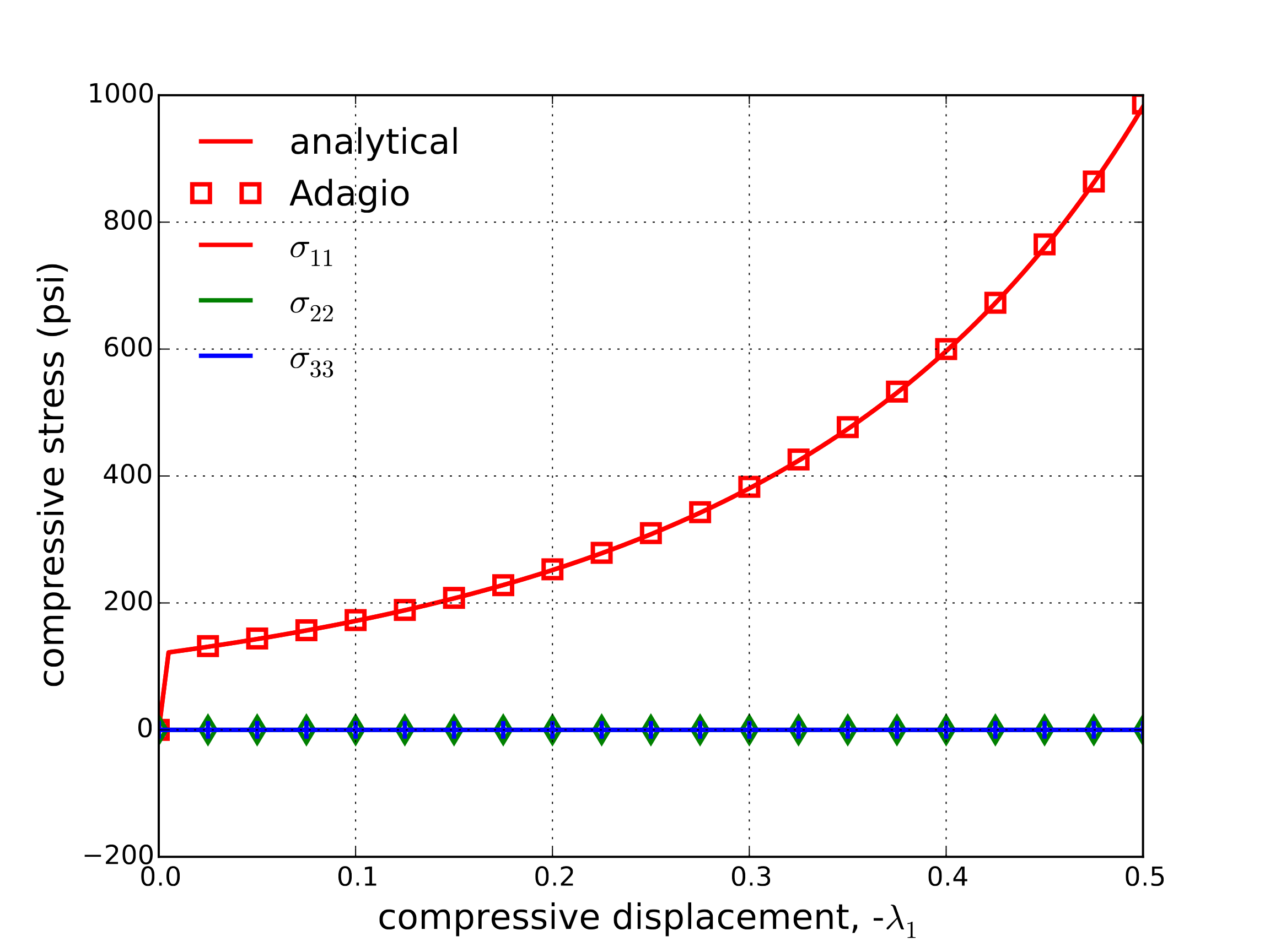
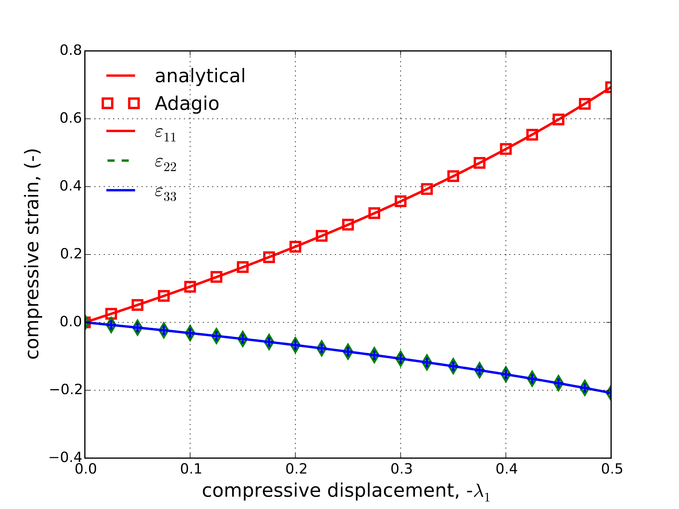
4.34.3.1. Uniaxial Compression

First, the case of uniaxial compression is treated to investigate the hardening behavior. As a uniaxial compressive stress state is being explored, the principal stresses are simply \(\sigma^1=\sigma^2=0\) and \(\sigma^3=\sigma_{11}\) enabling the development of analytical solutions. To this end, \(u_1=\lambda_1\) and the remaining surfaces are left traction free. The corresponding strain state is then,

\[\begin{split}\varepsilon_{11} & = \ln\left(1+\lambda_1\right), \\ \varepsilon_{22} = \varepsilon_{33} & = -\nu\ln\left(1+\lambda_1\right), \nonumber\end{split}\]

producing a engineering volume strain of,

\[\varepsilon_{\text{V}}=\left(1+\lambda_1\right)^{\left(1-2\nu\right)}-1.\]

Noting the elastic uniaxial stress, \(\hat{\sigma}_{11}\), is simply,

\[\hat{\sigma}_{11}=\left[\lambda\left(1-2\nu\right)+2\mu\right]\ln\left(1+\lambda_1\right),\]

the final stress state is simply \(\sigma_{22}=\sigma_{33} = 0\) and,

\[\begin{split}\sigma_{11} = \left\{\begin{array}{cc} \hat{\sigma}_{11} & \hat{\sigma}_{11} \leq -ae^{-b\varepsilon_{\text{V}}} \\ -ae^{-b\varepsilon_{\text{V}}} & \hat{\sigma}_{11} > -ae^{-b\varepsilon_{\text{V}}} \end{array}\right. .\end{split}\]

The analytical and numerical solution (from adagio) of this problem are presented in Fig. 4.145 with the stress and strains given in Fig. 4.145(a) and Fig. 4.145(b), respectively. Excellent agreement is observed verifying the compressive hardening performance.

Linear, Johnson-Cook

Linear, Power-Law Breakdown

Fig. 4.145 Analytical and numerical results of the normal stress and strain components through a compressive uniaxial stress loading path as a function of the applied displacement, \(\lambda_1\)

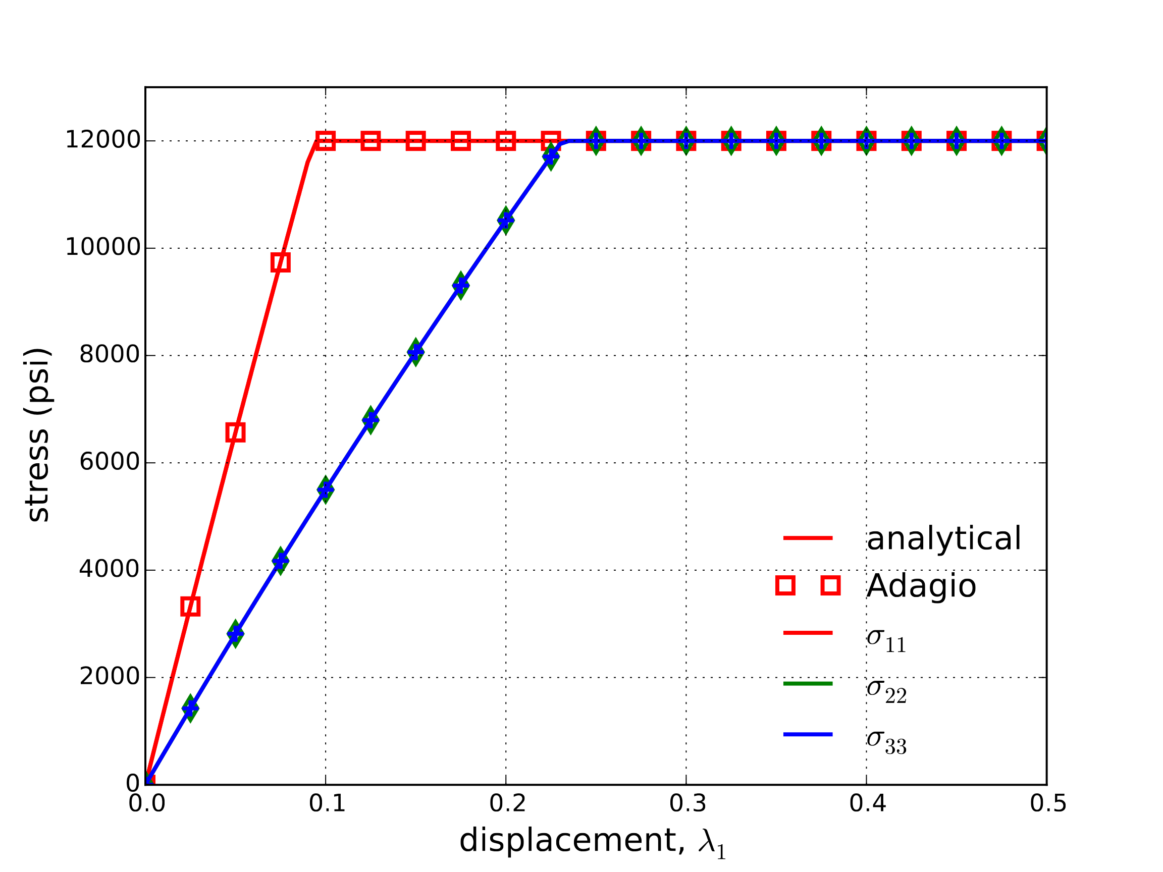
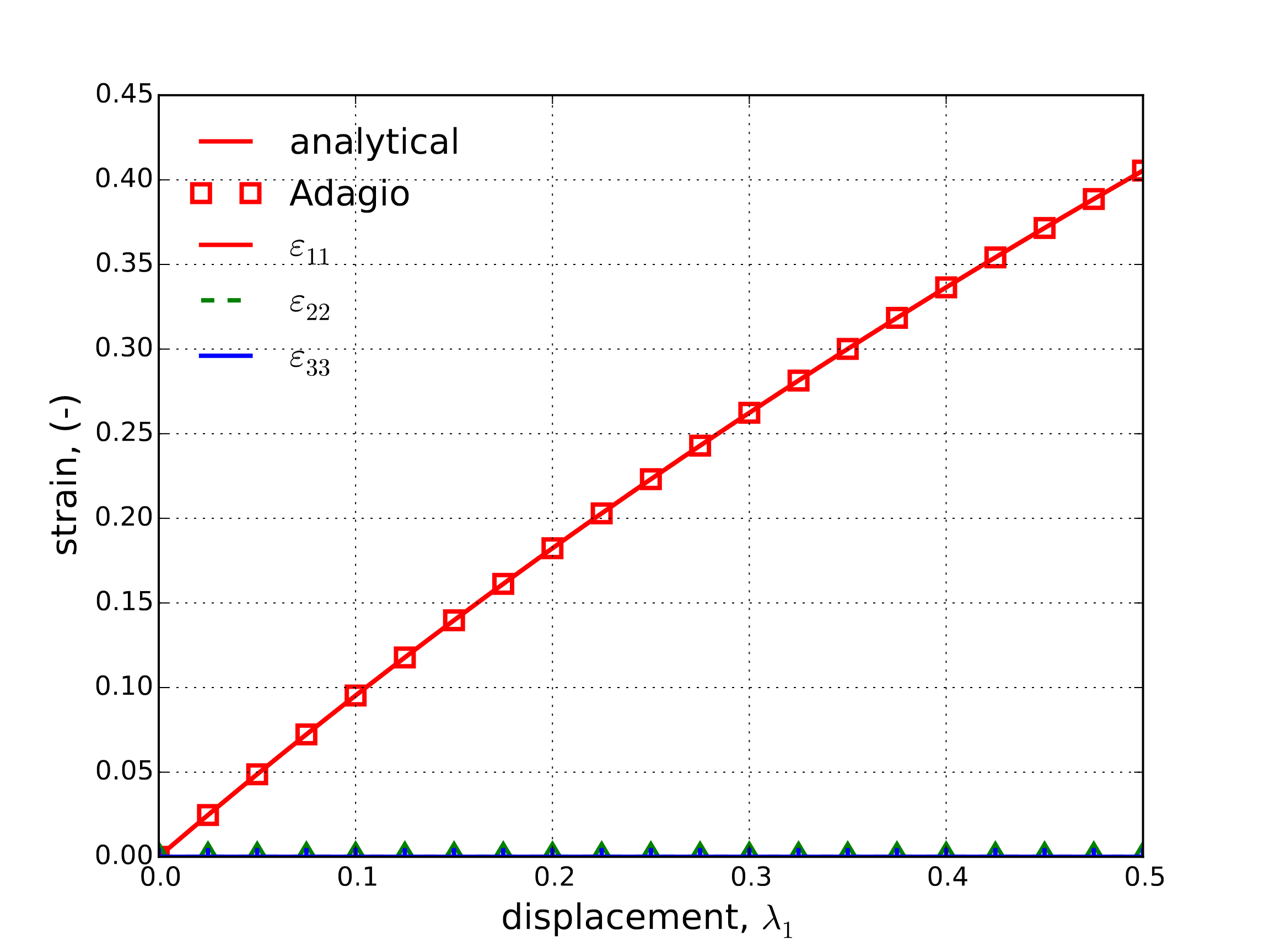
4.34.3.2. Uniaxial Tension

To consider the tensile behavior, the response of the model under a uniaxial tensile emph{strain} loading is interrogated. In this case the applied displacement is \(u_i = \lambda_1\delta_{i1}\) with the remaining displacements fixed such that \(\varepsilon_{22}=\varepsilon_{33}=0\) and the axial strain is again \(\varepsilon_{11}=\ln\left(1+\lambda_1\right)\). Given that the model behavior is perfectly plastic after yield, the axial and off-axis responses both reduce to bilinear forms. As such, the applied deformation necessary to induce the perfectly plastic response in the axial direction, \(\lambda_1^{\text{crit}}\), is simply

\[\lambda_1^{\text{crit}} = e^{\tau/\left(\lambda+2\mu\right)}-1,\]

leading to an expression for the axial stress as,

\[\begin{split}\sigma_{11} = \left\{\begin{array}{cc} \left(\lambda+2\mu\right)\ln\left(1+\lambda_1\right) & \lambda_1 < \lambda_1^{\text{crit}} \\ \tau & \lambda_1 \geq \lambda_1^{\text{crit}}\end{array}\right. .\end{split}\]

For the off-axis behavior, the critical displacement, \(\lambda_1^{\text{off-crit}}\), is

\[\lambda_1^{\text{off-crit}} = e^{\tau/\lambda}-1,\]

producing stresses of the form,

\[\begin{split}\sigma_{22}=\sigma_{33}=\left\{\begin{array}{cc} \lambda\ln\left(1+\lambda_1\right) & \lambda_1 < \lambda_1^{\text{off-crit}} \\ \tau & \lambda_1 \geq \lambda_1^{\text{off-crit}} \end{array}\right. .\end{split}\]

The stress and strain responses (both numerical and analytical) are presented below in Fig. 4.146(a) and Fig. 4.146(b), respectively, and excellent agreement is observed verifying this behavior in this deformation mode.

Linear, Johnson-Cook

Linear, Power-Law Breakdown

Fig. 4.146 Analytical and numerical results of the normal stress and strain components through a tension uniaxial strain loading path as a function of the applied displacement, \(\lambda_1\).

4.34.3.3. Hydrostatic Compression

To further explore the compressive response, the models behavior under a hydrostatic (compressive) loading is investigated. In this instance, the corresponding stress state produces a single, repeated, principal stress associated with the pressure, \(p=-\left(1/3\right)\sigma_{kk}\) (here defined positively in compression). Details of this loading may be found in Appendix A, although in this instance it is important to point out that,

\[\varepsilon_{\text{V}}=\left(1+\lambda_1\right)^3-1,\]

and the stress state reduces to,

\[p = -3K\ln\left(1+\lambda_1\right)\]

in the elastic limit and

\[p = ae^{-b\varepsilon_{\text{V}}},\]

during plastic loading. The numerical and analytical results are presented in Fig. 4.147 and excellent agreement in noted.

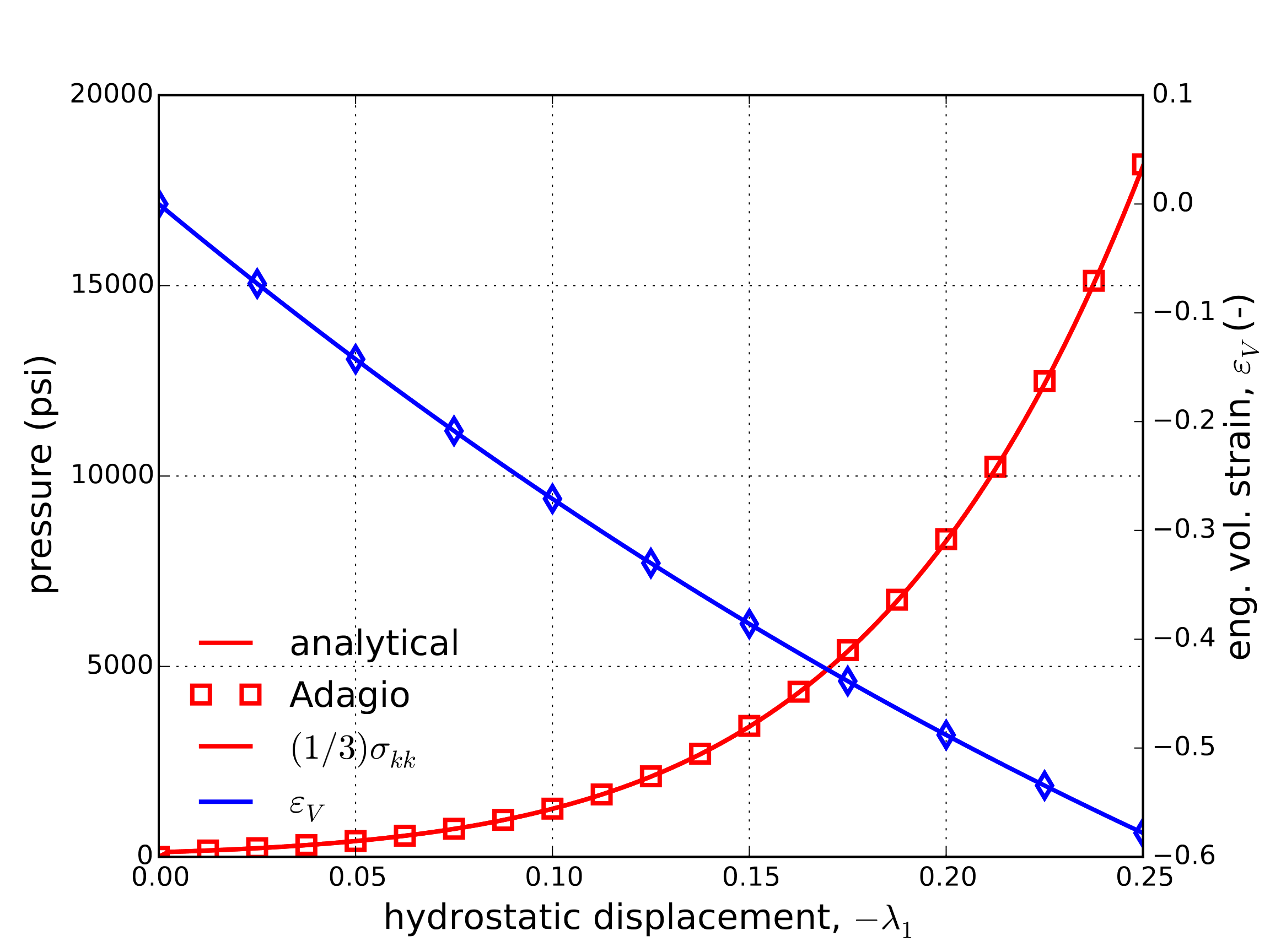
Fig. 4.147 Analytical and numerical pressure-volume strain response of the wire mesh model through a hydrostatic compression loading as a function of the applied displacement, \(\lambda_1\).

4.34.4. User Guide

BEGIN PARAMETERS FOR MODEL WIRE_MESH
  #
  # Elastic constants
  #
  YOUNGS MODULUS = <real>
  POISSONS RATIO = <real>
  SHEAR MODULUS  = <real>
  BULK MODULUS   = <real>
  LAMBDA         = <real>
  TWO MU         = <real>
  #
  # Yield surface parameters
  #
  YIELD FUNCTION = <string>
  TENSION        = <real>
END [PARAMETERS FOR MODEL WIRE_MESH]

• The yield function in compression is defined with the YIELD FUNCTION command line.

• The tensile strength is give by the TENSION command line.

Output variables available for this model are listed in Table 4.57.

More information on the model can be found in the report by Neilsen, et. al. [[1]].

Table 4.57 State Variables for WIRE MESH Model

Name	Description
EVOL	engineering volumetric strain
YIELD	current yield strength in compression

---

[1] (1,2,3,4,5)

M.K. Neilsen, J.D. Pierce, and R.D. Krieg. A constitutive model for layered wire mesh and aramid cloth fabric. Technical Report SAND91-2850, Sandia National Laboratories, Albuquerque, NM, 1993. \href http://infoserve.sandia.gov/sand_doc/1991/912850.pdfpdf.

[2]

M.K. Neilsen, H.S. Morgan, and R.D. Krieg. A phenomenological constitutive model for low density polyurethane foams. Technical Report SAND86-2927, Sandia National Laboratories, Albuquerque, NM, April 1987. \href http://infoserve.sandia.gov/sand_doc/1986/862927.pdfpdf.

[3]

W.M. Scherzinger and C.R. Dohrmann. A robust algorithm for finding the eigenvalues and eigenvectors of 3x3 symmetric matrices. Computer Methods in Applied Mechanics and Engineering, 197(45-48):4007–4015, 2008.