4.32. Universal Polymer Model

4.32.1. Theory

The Universal Polymer Model (UPM) is a phenomenological, non-linear viscoelastic (NLVE) model that is, in the literature, named the Simplified Potential Energy Clock (SPEC) [[1]]. The UPM model is considerably simpler than the parent model, the Potential Energy Clock (PEC) model, labeled the NLVE polymer model in SIERRA, which itself is not phenomenological but requires extensive data and experience to calibrate [[2]].

The UPM model is suitable for modeling the finite deformation, thermal-mechanical behavior of glassy materials, both organic and inorganic. Successful usage of the model is widespread. Some examples include the modeling of amorphous, thermosetting polymers across and through the glass transition such as epoxies [[3]]. It is also suitable for modeling thermoplastics from within the melt state and down into the glass transition from polystyrene to polycarbonate. Finally, it has been used to represent inorganic glasses for glass-to-metal seals. The UPM model was developed for production analyses of encapsulated components. It predicts a full range of behavior including yielding, stress relaxation, volume relaxation, and physical aging.

The key physical principal behind the UPM model is that there exists a material time scale (material clock) separate from the laboratory time scale. If the material time scale is fast, such as in the rubbery state of a polymer, then the UPM model responds instantly to changes in temperature and strain such that the user would observe rate-independent behavior. However, if the material clock is slow relative to the laboratory time scale, viscoelastic memory builds with any process, which causes acute history and thermodynamic path dependent behavior.

The model response is derived from a Helmholtz Free Energy density and takes as an input the unrotated rate of deformation, \(d_{ij}\), the temperature at the start and end of the time step (\(\theta_{n}\) and \(\theta_{n+1}\), and the time step, \(\Delta\,t\). From these inputs, the hereditary integrals within the model are updated, and the unrotated Cauchy stress tensor is returned.

For the UPM model, the strain measure is approximated from the integrated unrotated rate of deformation tensor, which we label \(\epsilon_{ij}\),

(4.149)\[ \epsilon_{ij} = \int_{0}^{\infty} \left( R_{mi}D_{mn} R_{nj} \right) ds, \quad D_{ij} = \frac{1}{2}\left( L_{ij} + L_{ji}\right), \quad F_{ij} = R_{im} U_{mj}.\]

Here, \(F_{ij}\), \(R_{ij}\), \(U_{ij}\), \(L_{ij}\), and \(D_{ij}\) are the deformation gradient, rotation, material stretch, velocity gradient, and rate of deformation tensors standard in Lagrangian continuum mechanics.

The UPM model allows the user to initiate an analysis from a stress-free temperature, \(\theta_{\rm sf}\), that is different from the reference temperature, \(\theta_{\rm ref}\), at which all material properties are defined. Here we briefly summarize the constitutive equations. The model is derived from a Helmholtz Free Energy, but we begin directly with the (unrotated) Cauchy Stress and refer the reader to reference [[1]] for more detail:

(4.150)\[\begin{split}\sigma_{ij} = \left( K_{G}\left( \theta \right) - K_{\infty} \left( \theta \right) \right) \int_{0}^{t}{f_v\left(t' - s'\right)}\frac{d I_1}{ds}{ds}\delta_{ij} \\ - \left(K_{G}\left( \theta \right) \delta_{G}\left(\theta\right) - K_{\infty} \left(\theta\right)\delta_{\infty} \left(\theta\right) \right) \int_{0}^{t}{f_v\left( t' - s'\right)}\frac{d \theta}{ds}{ds}\delta_{ij} \\ +2 \left( G_{G}\left( \theta \right) - G_{\infty} \left(\theta \right) \right) \int_{0}^{t}{f_{s}\left(t' - s'\right)} \frac{d \left( {\rm dev} \epsilon_{ij} \right)}{ds} ds \\ + \left( K_{\infty} \left( \theta \right) I_1 - K_{\infty} \left( \theta \right) \delta_{\infty} \left( \theta \right) \left( \theta - \theta_{\rm sf} \right) \right) \delta_{ij} + 2 G_{\infty} \left( \theta \right) {\rm dev} \epsilon_{ij}.\end{split}\]

The first three lines of terms in (4.150) represent the time-dependent and dissipative (non-equilibrium) response of the model to volumetric, thermal, and shear deformation histories. Accordingly, \(K\), \(\delta\), and \(G\) represent a bulk modulus, volumetric thermal expansion coefficient, and shear modulus while subscripts \(_G\) or \(_\infty\) denote a glassy or rubbery, respectively, properties. The last collection of terms in (4.150) furnish the time-independent rubbery (equilibrium) response. The variables in (4.150) are:

(4.151)\[\begin{split}I_1 & = \delta_{ij}\epsilon_{ij} = {\rm tr} \epsilon_{ij}, \qquad\qquad\quad {\rm dev}\epsilon_{ij} = \epsilon_{ij} - \frac{ I_1 }{3}\delta_{ij} , \\ G_G \left( \theta \right) & = G_G^{\rm ref} + \frac{dG_G}{d\theta} \left( \theta - \theta_{\rm ref}\right) , \quad G_\infty \left( \theta \right) = G_\infty^{\rm ref} + \frac{dG_\infty}{d\theta} \left( \theta - \theta_{\rm ref}\right) , \\ K_G \left( \theta \right) & = K_G^{\rm ref} + \frac{dK_G}{d\theta} \left( \theta - \theta_{\rm ref}\right) , \quad K_\infty \left( \theta \right) = K_\infty^{\rm ref} + \frac{dK_\infty}{d\theta} \left( \theta - \theta_{\rm ref}\right) , \\ \delta_G \left( \theta \right) & = \delta_G^{\rm ref} + \frac{ d \delta_G}{d\theta} \left( \theta - \theta_{\rm ref}\right) , \quad \delta_\infty \left( \theta \right) = \delta_\infty^{\rm ref} + \frac{ d \delta_\infty}{d\theta} \left( \theta - \theta_{\rm ref}\right).\end{split}\]

The first three terms in (4.150) represent the material’s viscoelastic response to changes in volume strain, temperature, and shear deformation. Two relaxation functions are used to characterize the thermal/volumetric (\(f_v\)) and shear (\(f_v\)) relaxation responses. The model assumes the thermal and volumetric relaxation responses are identical. Otherwise, \(f_v\) and \(f_s\) are typically quite different and are expressed as a Prony series (Note: to distinguish between indices used with conventional summation convention and those related to Prony series terms, all Prony series summations shall be explicitly written with the relevant index given parenthetically in a superscript.):

(4.152)\[f_v\left(x\right) = \sum_{k=1}^{N} w^{\left(k\right)} \exp \left( -\frac{x}{\tau^{\left(k\right)}} \right), \quad f_s\left(x\right) = \sum_{l=1}^{M} w^{\left(l\right)} \exp \left( -\frac{x}{\tau^{\left(l\right)}} \right).\]

These relaxation functions describe the material’s response to a suddenly applied volumetric/thermal or shear perturbation at the reference temperature where, under certain conditions, the material and laboratory time scales are equivalent. In (4.150), the viscous terms (non-rubbery) involve hereditary integrals over the difference in material time from \(s=0\) to \(s=t\), which is the current laboratory time.

An increment in material time, \(dt'\), and the laboratory time, \(dt\), are related through the (highly) history dependent shift factor, \(a\), such that the difference in material time, \(t' - s'\), is related to the corresponding difference in laboratory time, \(t - s\) through:

(4.153)\[a dt' = dt, \quad t' - s' = \int_{u=s}^{u=t} \frac{du}{a\left(u\right)}.\]

If the material time scale is very slow compared to the laboratory time, then \(a>>1\), which is often the case inside and below the glass transition for typically glassy materials.

The shift factor is instantaneously defined through:

(4.154)\[\begin{split}{\rm log_{10}} a & = \frac{-C_1 N}{ C_2 + N }, \\ N(t) & =\theta - \theta_{\rm ref} - \int_0^t f_v\left( t' - s' \right) \frac{d\theta}{ds}ds \\ & + C_3 \left( I_1 - \int_0^t f_v\left( t' - s' \right) \frac{d I_1}{ds}ds \right) \\ & + C_4 \int_{u=0}^{u=t} \int_{s=0}^{s=t} \left( f_{s}\left( t' - s' , t' - u' \right)\frac{d \left( {\rm dev}\epsilon_{ij} \right)}{ds}\frac{d \left( {\rm dev} \epsilon_{ij} \right)}{du} ds du \right).\end{split}\]

The key physics in the model comes from (4.154). Temperature rise (generally) causes \(N\) to increase, and hence the material shift factor shrinks (the material time scale speeds up). Shrinking the volume generally causes the shift factor to increase as if the temperature had been decreased. Mechanistically, this feature is the manifestation of the trade-off between between mobility and free volume available to polymer chains. Finally, shear deformation can greatly speed up the material clock through the last term. This phenomenon is a direct manifestation of deformation induced mobility, a key mechanism for glassy materials.

Since the shift factor involves hereditary integrals, even at a constant temperature and state of deformation, the material clock will change over time. Under stress-free conditions, the material will creep and densify if the model is out of equilibrium (when any viscous term is non-zero). These phenomena are the model’s manifestations of physical aging, time-dependent material change without a change in composition or microstructure. \(C_1\), \(C_2\), \(C_3\), and \(C_4\) are all material constants. We note that the double relaxation function appearing in the last term takes on a slightly different form from \(f_s\):

(4.155)\[ f_{s}\left( x, y \right) = \sum_{k=1}^{N} w^{\left(k\right)} \exp\left( -\frac{x}{\tau^{\left(k\right)}} \right) \exp\left( -\frac{y}{\tau^{\left(k\right)}} \right)\]

It is desirable to relate a special case of the model to the Williams-Landel-Ferry (WLF) form because of how time-temperature superposition fitting is typically performed. Specifically, one can show that the clock parameters, \(C_1\) and \(C_2\), relate to the WLF parameters, \(\hat{C}_1\) and \(\hat{C}_2\), through the following relationships: \(\hat{C}_1 = C_1\) and \(\hat{C}_2 = C_2 /\left(1 + C_3 \delta_{\infty}^{\rm ref} \right)\).

For more information about the universal polymer model, consult [[1]].

4.32.2. Implementation

The hereditary integrals in (4.150) and (4.154) are difficult to evaluate directly. Instead a rate form is pursued than can be integrated straightforwardly over each time step. Consider a typical hereditary integral after the Prony series for its specific relaxation function has been substituted into it. Differentiate the integral with respect to the current time, \(t\), and use the Leibnitz rule to arrive at:

(4.156)\[\int_{s=0}^{s=t} f_v\left(t' - s'\right) \frac{d\theta}{ds}ds = \sum_{k=0}^{N} w^{\left(k\right)} \int_{s=0}^{s=t} \exp\left( -\frac{t' - s'}{\tau^{\left(k\right)}} \right) \frac{d\theta}{ds}ds = \sum_{k=0}^{N} w^{\left(k\right)} J^{\left(k\right)}\]

\[\begin{split}\frac{d J^{\left(k\right)}}{dt} & = \int_{s=0}^{s=t} \frac{d}{dt} \left( \exp\left( -\frac{t' - s'}{\tau^{\left(k\right)}} \right) \frac{d\theta}{ds} \right) ds + \left( \exp\left( -\frac{t' - s'}{\tau^{\left(k\right)}} \right) \frac{d\theta}{ds} \right)_{s=t} \frac{d(t)}{dt} \\ & =\int_{s=0}^{s=t} \exp\left(-\frac{t' - s'}{\tau^{\left(k\right)}}\right) \frac{d\theta}{ds} \left(\frac{-1}{\tau^{\left(k\right)}}\right) \frac{d t'}{dt} ds + \frac{d\theta}{dt} \\ & = -\frac{1}{a \tau^{\left(k\right)}} J^{\left(k\right)} + \frac{d\theta}{dt}.\end{split}\]

Notice this rate form involves a memory term which decays as well as input from new history, in this case a change in temperature. To integrate this easily, we approximate this rate as constant over the time step in a constitutive equation update and use the mid-step evaluation to determine the rate. Consider a process in which the temperature changes from \(\theta_n\) at time \(t_n\) to \(\theta_{n+1}\) at \(t_{n+1}\) so that \(\Delta t = t_{n+1} - t_{n}\). Then,

(4.157)\[\frac{d J^{\left(k\right)}}{dt}\vert_{t_{n+1/2}} \approx \frac{J^{\left(k\right)} \left(t_{n+1} \right) - J^{\left(k\right)}\left( t_n \right)}{t_{n+1} - t_{n}} = -\frac{1}{a_{t_{n+1/2}} \tau^{\left(k\right)}} \frac{J^{\left(k\right)}\vert_{n+1} + J^{\left(k\right)}\vert_{n}}{2} + \frac{\theta_{n+1} - \theta_{n}}{t_{n+1} - t_{n}},\]

yielding,

\[J^{\left(k\right)}\vert_{n+1} = \left( \frac{ 2 a_{n+1/2} \tau^{\left(k\right)} - \Delta t }{2 a_{n+1/2} \tau^{\left(k\right)} + \Delta t} \right) J^{\left(k\right)}\vert_{n} + \left( \frac{ 2 a_{n+1/2} \tau^{\left(k\right)} }{2 a_{n+1/2} \tau^{\left(k\right)} + \Delta t} \right) \left( \theta_{n+1}- \theta_{n} \right).\]

Stability of (4.157) requires that the first term to remain positive. Hence, the change in time for the purposes of updating these hereditary integrals is:

(4.158)\[\Delta t = {\rm MIN} \left( t_{n+1} - t_n, 2 a_{n+1/2} \tau^{\left(k\right)} \right).\]

The collection of \(J^{\left(k\right)}\) from \(k=1,N\) are internal state variables associated with this particular hereditary integral. Each Prony term for each distinct hereditary integral must be stored as an internal state variable.

Fortunately, changing from a scalar field to a tensor field (\(\theta\) to \(\epsilon_{ij}\)) does not alter the above time integration except that for each Prony term, each component of the tensor must be stored and updated as a state variable. For example, the hereditary integrals associated with deviatoric strain history may be updated by letting,

(4.159)\[H_{ij} = \int_{0}^{t}{ds}{f_{s}\left(t' - s'\right)}\frac{d \left( {\rm dev} \epsilon_{ij} \right)}{ds} ds = \sum_{k=1}^{N} w^{\left(k\right)} H_{ij}^{\left(k\right)},\]

and approximating the time rate of change at the midstep as,

\[\frac{d H_{ij}^{\left(k\right)}}{dt}\vert_{t_{n+1/2}} \approx \frac{ H_{ij}^{\left(k\right)} \left(t_{n+1} \right) - H_{ij}^{\left(k\right)}\left( t_n \right)}{t_{n+1} - t_{n}} = -\frac{1}{a_{t_{n+1/2}} \tau^{\left(k\right)}} \frac{H_{ij}^{\left(k\right)}\vert_{n+1} + H_{ij}^{\left(k\right)}\vert_{n}}{2} + \frac{H_{ij}^{n+1} - H_{ij}^{n}}{t_{n+1} - t_{n}},\]

resulting in,

\[H_{ij}^{\left(k\right)}\vert_{n+1} = \left( \frac{ 2 a_{n+1/2} \tau^{\left(k\right)} - \Delta t }{2 a_{n+1/2} \tau^{\left(k\right)} + \Delta t} \right) H_{ij}^{\left(k\right)}\vert_{n} + \left( \frac{ 2 a_{n+1/2} \tau^{\left(k\right)} }{2 a_{n+1/2} \tau^{\left(k\right)} + \Delta t} \right) \left( H_{ij}^{n+1} - H_{ij}^{n} \right).\]

Here, \(H_{ij}^{\left(k\right)}\) is a collection of six state variables that compose the \(k^{\rm th}\) Prony term deviatoric strain history hereditary integral as in (4.150). The superscripts refer to the Prony term number, and each component of these tensors much be updated and stored.

Because of the double hereditary integral in (4.154) associated with shear deformation and shift factor acceleration, a rate form for this kind of term is also needed. Again, differentiate the integral with respect to the current time, \(t\), and use the Leibnitz rule to arrive at:

(4.160)\[\begin{split}\int_{u=0}^{u=t} \int_{s=0}^{s=t} \left( f_{s}\left( t' - s' , t' - u' \right)\frac{d \left( {\rm dev}\epsilon_{ij} \right)}{ds}\frac{d \left( {\rm dev} \epsilon_{ij} \right)}{du} ds \,du \right) \\ = \sum_{k=1}^{N} w^{\left(k\right)} \int_{u=0}^{u=t} \int_{s=0}^{s=t} \left( \exp\left(-\frac{t' - s'}{\tau^{\left(k\right)}} \right) \exp\left(- \frac{ t' - u' }{\tau^{\left(k\right)}} \right) \frac{d \left( {\rm dev} \epsilon_{ij} \right)}{ds}\frac{d \left( {\rm dev} \epsilon_{ij} \right)}{du} ds \,du \right) \nonumber \\ = \sum_{k=0}^{N} w^{\left(k\right)} Q^{\left(k\right)} .\nonumber\end{split}\]

\[\begin{split}\frac{d Q^{\left(k\right)}}{dt} & = \frac{-2 Q^{\left(k\right)}}{a \tau^{\left(k\right)}} + 2 \frac{d \left( {\rm dev} \epsilon_{ij} \right)}{dt}\int_{s=0}^{s=t} \left(\exp\left( - \frac{ t' - u' }{\tau^{\left(k\right)}} \right) \frac{d \left( {\rm dev} \epsilon_{ij} \right)}{du} du \right) \\ & = \frac{-2 Q^{\left(k\right)}}{a \tau^{\left(k\right)}} + 2 \frac{d \left( {\rm dev}\epsilon_{ij} \right)}{dt}H_{ij}^{\left(k\right)}. \nonumber\end{split}\]

The variables \(J^{\left(k\right)}\), \(Q^{\left(k\right)}\), and all six components of \(H_{ij}^{\left(k\right)}\) are state variables that are stored and updated through the midstep algorithm presented above.

The actual update of the constitutive equations involves finding the shift factor at \(t_{n+1/2}\), which requires Newton’s method on (4.154). Using the techniques from (4.156) through (4.160), it is straightforward to chain rule differentiate the term \(N\) in (4.154), and that analysis is not reproduced here for brevity.

4.32.3. Verification

Verification for the full non-linear viscoelastic features of the universal polymer model is difficult because analytic solutions are not available. Here we verify that two key parts of the model are working correctly, but at this time not all non-linearities in the material clock are verified. First, we verify that the material clock (shift factor) follows the Williams-Landel-Ferry behavior near and above the glass transition (reference temperature). Then, as the material is cooled below the glass transition, we verify that the thermal hereditary integral in the material clock is working properly. Finally, the specimen is reheated through the glass transition, and the shift factor is again compared between the UPM model and a semi-analytic solution.

Second, with the non-linear portions of the clock turned off and the temperature held fixed, an analytic solution to the uniaxial strain boundary value problem is pursued at three different strain rates. This latter verification exercise demonstrates that the hereditary integrals are updated correctly and that the stress response may be calculated using both the shear and bulk relaxation responses simultaneously even when they have different relaxation functions.

4.32.3.1. Shift Factor During Traction-Free Cooling and Heating

The WLF equation (considering temperature only) provides a simple means of performing time-temperature superposition. It relates the shift factor, \(a\), to the current temperature through,

(4.161)\[\log_{10} a = -\frac{C_1\left( \theta - \theta_{\text{ref}} \right)} { C_2 + \left( \theta - \theta_{\text{ref}} \right)}.\]

Near and above \(\theta_{\text{ref}}\), the UPM model limits to the WLF model, and below the glass transition, the hereditary integral in the clock freezes out further evolution of the shift factor with temperature.

A single element boundary value problem is analyzed in Sierra/SM with the UPM model. A simple temperature sweep is executed under traction free conditions through the glass transition starting from above it at a constant rate of 1\(^{\circ}\)C per minute. The material is then immediately reheated at 1\(^{\circ}\)C per minute to well above the glass transition. The material properties used for this analysis as well as the uniaxial strain problem below are provided in Table 4.51 and reflect a simplified version of the material properties used to represent 828DGEBA / DEA (often called 828DEA) [[1]].

Table 4.51 The material and model parameters for the Universal Polymer Model used for verification testing. Parameters are approximately based on a fit for 828DEA, but they represent a linear thermal-viscoelastic representation of the model. Both the shear and volumetric Prony series weights come from fitting these 4 relaxation times to stretched exponential series as discussed in that paper. The thermal relaxation and volumetric relaxation functions are the same in the UPM model. All other material and model parameters are unused and set to zero.

\(\theta_{\text{ref}}\)	75\(^{\circ}\)C	\(\theta_{\text{sf}}\)	125\(^{\circ}\)C
\(\hat{C}_1\)	16.5	\(\hat{C}_2\)	54.5\(^{\circ}\)C
\(K_G\)	4.9 GPa	\(K_{\infty}\)	3.2 GPa
\(G_G\)	0.75 GPa	\(G_{\infty}\)	4.5 MPa
\(\left\{f_1\right\}\)	\(\{2.99149\times 10^{-3},\) \(6.42966\times 10^{-2},\) \(6.49783\times 10^{-1},\) \(2.82929\times 10^{-1}\}\)
\(\left\{f_2\right\}\)	\(\{1.00305\times 10^{-2},\) \(2.11421\times 10^{-1},\) \(7.01534\times 10^{-1},\) \(7.70145\times 10^{-2}\}\)
\(\left\{\tau\right\}\)	\(\{1.0\times 10^{-11},\) \(1.0\times 10^{-6},\) \(1.0\times 10^{-1},\) \(1.0\times 10^4 \}\) (s)

For the verification of the time-temperature shift behavior, the model is expected to exactly match the WLF behavior above \(\theta_{\text{ref}}\), but as the material is cooled below this point, the temperature hereditary integral in the material shift factor definition (4.154) slows further evolution of the shift factor. WLF behavior is observed in the model, which confirms this elementary behavior of the model in Fig. 4.138. Then, as the model is further cooled below the glass transition, the UPM model is compared against a custom Newton-Raphson scheme for this boundary value problem (outside Sierra), and agreement is perfect. During reheat, one sees that the shift factor does not retrace the path through temperature space, and a large hysteresis is observed.

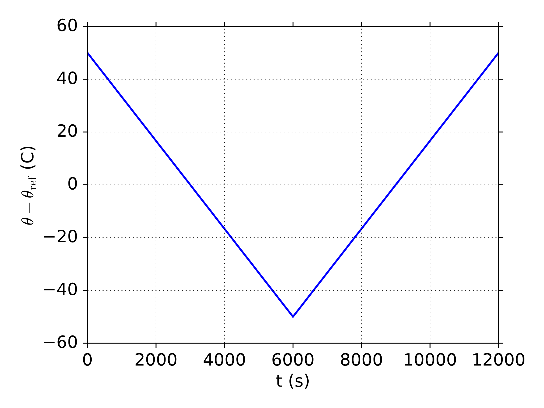Applied Temperature History

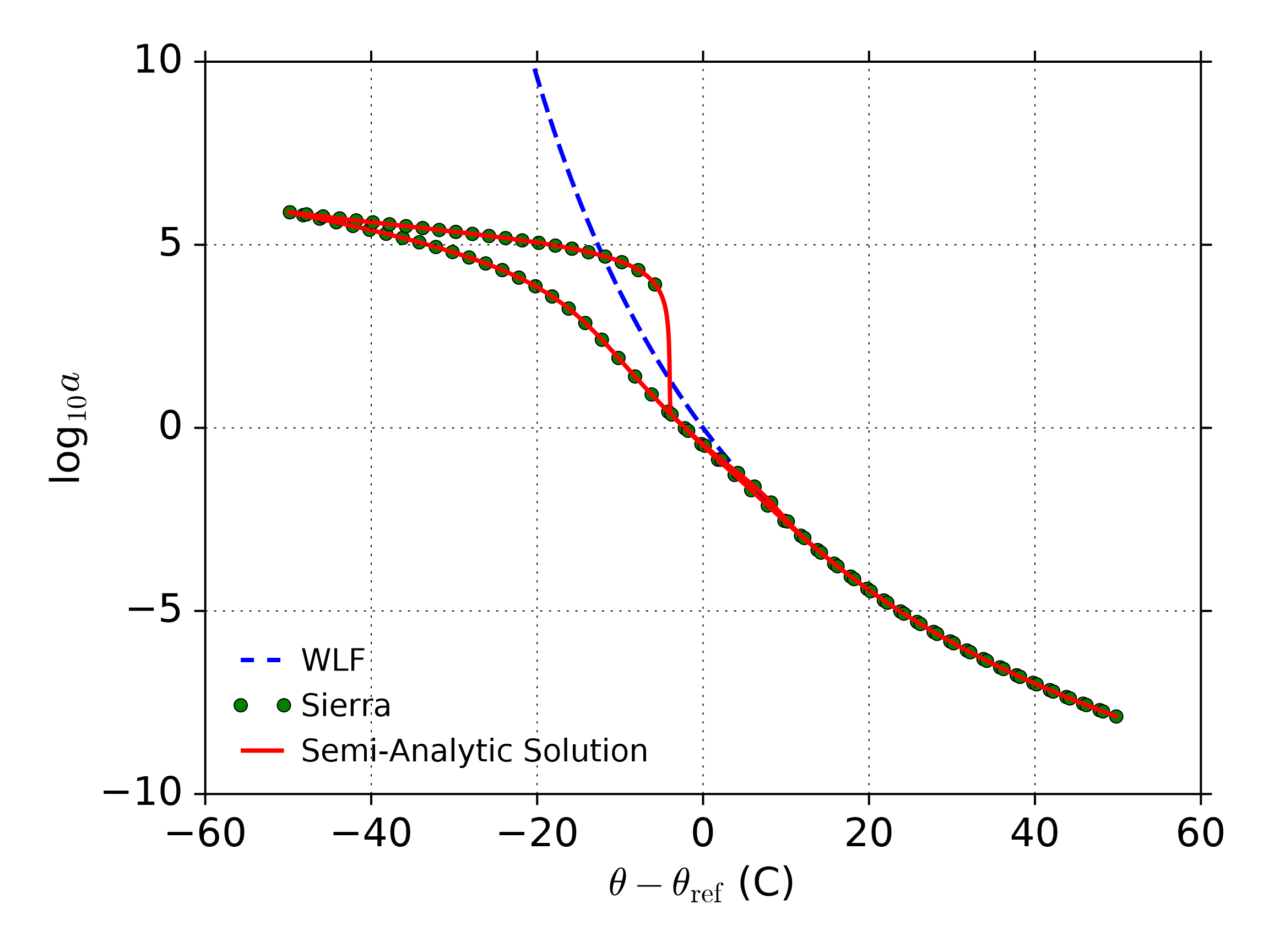Shift Factor Vs. Temperature

Fig. 4.138 Time-temperature dependence of the shift factor, \(a\), during cooling through the glass transition and then reheating back through it. The cooling/heating rate is 1\(^{\circ}\)C per minute. FEA (circles) show the expected WLF (blue dashed line) behavior for \(\theta-\theta_{\text{ref}} > 0\). The UPM model departs from WLF behavior below the reference temperature as expected, and continues to agree with an external to Sierra numerical scheme (solid line) to simulate this boundary value problem.

Changing the cooling rate changes the temperature at which the UPM model will depart from WLF behavior with the behavior remaining WLF like at colder temperatures for slower cooling rates and departing at warming temperatures for faster cooling rates.

4.32.3.2. Uniaxial Strain

The second verification problem considered is uniaxial strain under isothermal conditions wherein the non-linear clock terms are set to zero (\(C_3 = 0\) and \(C_4 = 0\)). Here, the temperature is set to the reference temperature, \(\theta = \theta_{\text{ref}}\), and a two stage boundary value problem is simulated. A material point (single 8-node hexahedral element with selective deviatoric spatial integration) is loaded at a constant logarithmic strain rate in uniaxial strain up to a prescribed logarithmic strain (characterized by a loading time, \(t_{\text{L}}\)). Then, the logarithmic strain rate is fixed to zero. The stress responses in the axial and transverse directions are output over time during this load and hold process. Three logarithmic strain rates are considered: 0.001, 1, and 1000 per second which activate the rubbery, mixed, and glassy responses respectively. For all three cases, the specimen is loaded to 10% axial logarithmic strain, and then the specimen is held for 10 seconds. Uniaxial strain involves finite volume and shape change, and so this boundary value problem tests both relaxation processes simultaneously.

Next we develop the analytic solution for linear thermal-viscoelasticity based on the UPM model. Note that the temperature is fixed to the reference temperature such that the shift factor is 1.0 always. We prescribe the following logarithmic strain rate history on a material point (in a Cartesian frame). Since both the spherical and deviatoric parts of the logarithmic strain history are needed for the model, we derive them too:

(4.162)\[\begin{split}{\text{for} \quad 0\leq t \leq t_{\text{L}}}, \quad\quad \dot{H}_{ij} = \dot{\epsilon} \begin{bmatrix} 1 & 0 & 0 \\ 0 & 0 & 0 \\ 0 & 0 & 0 \\ \end{bmatrix} ,\quad \dot{H}_{ij}^{\text{dev}} = \frac{\dot{\epsilon}}{3} \begin{bmatrix} 2 & 0 & 0 \\ 0 & -1 & 0 \\ 0 & 0 & -1 \\ \end{bmatrix}, \\ \nonumber {\text{otherwise}} \quad \quad \dot{H}_{ij} = \dot{H}_{ij}^{\text{dev}} = \begin{bmatrix} 0 & 0 & 0 \\ 0 & 0 & 0 \\ 0 & 0 & 0 \\ \end{bmatrix},\end{split}\]

and the associated strain invariants needed for the model are:

(4.163)\[\begin{split} I_1, \, I_2: \begin{cases} {\text{for} \quad 0\leq t \leq t_{\text{L}}}, \\ \quad\quad I_1 = \delta_{ij}H_{ij} = \dot{\epsilon} t \\ \quad\quad \dot{I}_1 = \dot{\epsilon} \\ \quad\quad I_2 = H_{ij}^{\text{dev}} H_{ij}^{\text{dev}} = \frac{2}{3} \dot{\epsilon}^{2}t^{2} \\ \quad\quad \dot{I}_2 = \frac{4}{3} \dot{\epsilon}^{2}t \\ \\ {\text{for} \quad t_{\text{L}} \leq t}, \\ \quad\quad I_1 = \dot{\epsilon} t_{\text{L}} \\ \quad\quad \dot{I}_1 = 0 \\ \quad\quad I_2 = \frac{2}{3} \dot{\epsilon}^{2}t_{\text{L}}^{2} \\ \quad\quad \dot{I}_2 = 0 \end{cases}\end{split}\]

Now, the motion involves a finite volume change, and the Jacobian of the deformation gradient will be needed. It is:

(4.164)\[\begin{split} J = \begin{cases} {\text{for} \quad 0\leq t \leq t_{\text{L}}}, \\ \quad \exp \left( \dot{\epsilon} t \right) % \\ % {\text{for} \quad t_{\text{L}} \leq t}, \\ \quad \exp \left( \dot{\epsilon} t_{\text{L}} \right) \end{cases}\end{split}\]

The derivation of the linear viscoelastic response proceeds directly with the stress integral from (4.150) with equivalent laboratory and material time scales since \(\theta = \theta_{\text{ref}}\). Using the prescribed strain history from (4.162) and the Jacobian of the deformation gradient (4.164), the Cauchy stress response is given below. Again, there are only two non-zero stress components: the axial stress (\(\sigma_{11}\)) and the transverse stresses (\(\sigma_{22}=\sigma_{33}\)), which we will label with under score \(\sigma_A\) and \(\sigma_T\) respectively. These are:

(4.165)\[\begin{split} {\text{for} \quad 0\leq t \leq t_{\text{L}}} : \begin{cases} J \sigma_{A} = \exp\left( -\dot{\epsilon} t \right) \\ ~~\qquad \left\{ \frac{4 \left(G_g - G_\infty\right) \dot{\epsilon}}{3} \sum_{k=1}^{N}w^{\left(k\right)} \tau^{\left(k\right)} \left( 1 - \exp\left( -\frac{t}{\tau^{\left(k\right)}}\right) \right) \right. \\ ~~\qquad \left. + \left( K_g - K_\infty \right) \dot{\epsilon} \sum_{l=1}^{M} q^{\left(l\right)} \tau^{\left(l\right)} \left( 1 - \exp\left( -\frac{t}{\tau^{\left(l\right)}}\right) \right) \right\} \\ ~~\qquad + \left( K_\infty + \frac{4}{3}G_\infty \right) \dot{\epsilon} t, \\ \\ J \sigma_{T} = \exp\left( -\dot{\epsilon} t \right) \\ ~~\qquad \left\{ -\frac{2 \left( G_g - G_\infty \right) \dot{\epsilon}}{3} \sum_{k=1}^{N}w^{\left(k\right)} \tau^{\left(k\right)} \left( 1 - \exp\left( -\frac{t}{\tau^{\left(k\right)}}\right) \right) \right.\\ ~~\qquad \left. + \left( K_g - K_\infty \right) \dot{\epsilon} \sum_{l=1}^{M} q^{\left(l\right)} \tau^{\left(l\right)} \left( 1 - \exp\left( -\frac{t}{\tau^{\left(l\right)}}\right) \right) \right\} \\ ~~\qquad + \left( K_\infty - \frac{2}{3}G_\infty \right) \dot{\epsilon} t, \end{cases}\end{split}\]

(4.166)\[\begin{split} {\text{for} \quad t_{\text{L}} \leq t} : \begin{cases} J \sigma_{A} = \exp\left( -\dot{\epsilon} t_{\text{L}} \right) \\ ~~\qquad \left\{ \frac{4 \left(G_g - G_\infty\right) \dot{\epsilon}}{3} \sum_{k=1}^{N}w^{\left(k\right)} \tau^{\left(k\right)} \left( \exp\left(-\frac{t-t_{\text{L}}}{\tau^{\left(k\right)}}\right)-\exp\left( -\frac{t}{\tau^{\left(k\right)}}\right) \right) \right. \\ ~~\qquad \left. + \left( K_g - K_\infty \right) \dot{\epsilon} \sum_{l=1}^{M} q^{\left(l\right)} \tau^{\left(l\right)} \left( \exp\left(-\frac{t-t_{\text{L}}}{\tau^{\left(l\right)}}\right)-\exp\left(-\frac{t}{\tau^{\left(l\right)}}\right) \right) \right\}\\ ~~\qquad + \left( K_\infty + \frac{4}{3}G_\infty \right) \dot{\epsilon} t_{\text{L}}, \\ \\ J \sigma_{T} = \exp\left( -\dot{\epsilon} t_{\text{L}} \right) \\ ~~\qquad\left\{ -\frac{2 \left( G_g - G_\infty \right) \dot{\epsilon}}{3} \sum_{k=1}^{N}w^{\left(k\right)} \tau^{\left(k\right)} \left(\exp\left(-\frac{t-t_{\text{L}}}{\tau^{\left(k\right)}}\right)-\exp\left(-\frac{t}{\tau^{\left(k\right)}}\right)\right) \right.\\ ~~\qquad\left. + \left( K_g - K_\infty \right) \dot{\epsilon} \sum_{l=1}^{M} q^{\left(l\right)} \tau^{\left(l\right)} \left(\exp\left( -\frac{t-t_{\text{L}}}{\tau^{\left(l\right)}}\right)-\exp\left(-\frac{t}{\tau^{\left(l\right)}}\right)\right) \right\}\\ ~~\qquad + \left( K_\infty - \frac{2}{3}G_\infty \right) \dot{\epsilon} t_{\text{L}}, \end{cases}\end{split}\]

Using the two Prony series in Table 4.51, and the three strain rates (0.1, 1, and 10 per second), the analytic model and UPM are directly compared in Fig. 4.139.

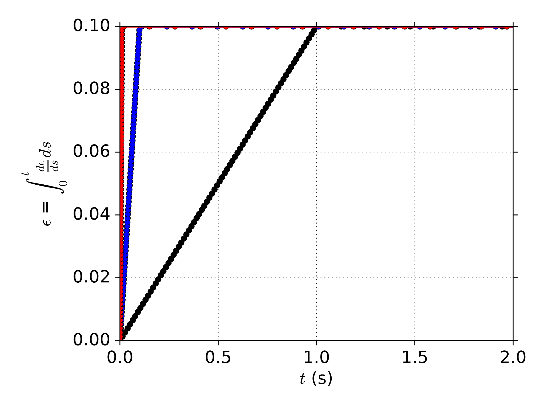Applied Strain History

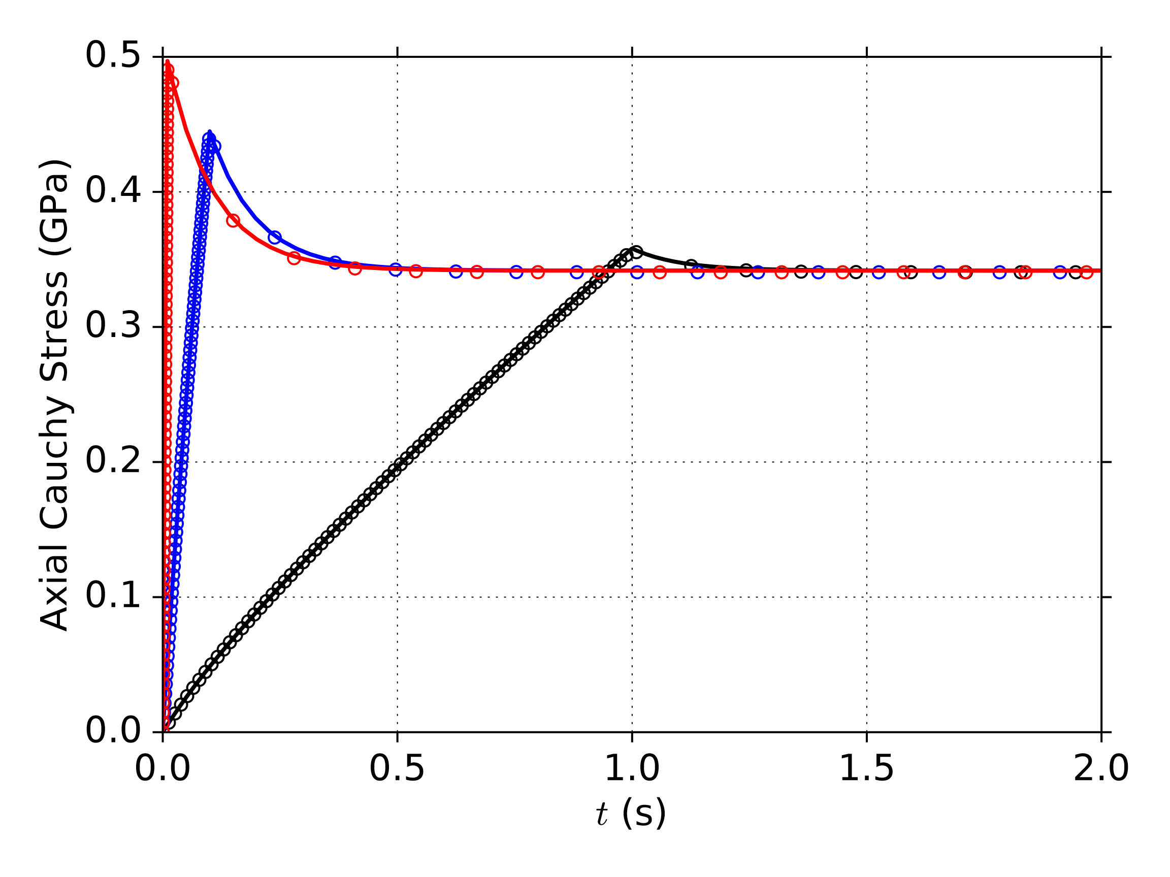Axial Stress History

Fig. 4.139 Linear viscoelastic response to a two stage uniaxial strain boundary value problem with material and loading properties specified in Table 4.51. Symbols represent FEA simulations with the UPM model while solid lines are the analytic results. The three logarithmic strain rates of 0.1, 1.0, and 10.0 per second are shown, and all cease at 10% strain, and all cases are isothermal at the reference temperature so that the shift factor is unity.

4.32.4. User Guide

The UPM model is commonly used in one of two ways. The most general use case is portrayed in full in the following syntax in which the user specifies both Prony series explicitly. That is, the user specifies all Prony relaxation times (\({\tau}\)) and weights for both the thermal/volumetric (\({f_v}\)) and shear (\({f_s}\)) relaxation functions. Note that in the UPM model, only a single set of Prony relaxation times can be specified and acts as the basis for both relaxation spectra. In other words, a single set of relaxation times is specified, and both functions use their own (distinct) weights.

Default parameters are not set. Any system of units can be used with the model. There are no internal units assumptions.

BEGIN PARAMETERS FOR MODEL UNIVERSAL_POLYMER
  #
  # Elastic constants: These Should be Set to the Glassy Moduli
  #                    for robustness considerations
  #
  SHEAR MODULUS  = <real>
  BULK MODULUS   = <real>
  #
  ## Reference Temperature and Material CLOCK Parameters
  #
  REFERENCE TEMPERATURE   = <real> # Temperature
  STRESS FREE TEMPERATURE = <real> # Temperature
  #
  WLF C1   = <real>
  WLF C2   = <real> # Temperature
  CLOCK C3 = <real> # Temperature
  CLOCK C4 = <real> # Temperature
  #
  ## Glassy and Rubbery Moduli
  #  and CTE Definitions at the Reference Temperature
  #
  BULK GLASSY 0    = <real> # Units of Pressure
  BULK RUBBERY 0   = <real> # Units of Pressure
  SHEAR GLASSY 0   = <real> # Units of Pressure
  SHEAR RUBBERY 0  = <real> # Units of Pressure
  VOLCTE glassy 0  = <real> # Units of Inverse Temperature
  VOLCTE rubbery 0 = <real> # Units of Inverse Temperature
  #
  FILLER VOL FRACTION = <real>
  #
  ## Relaxation Time Spectra Definitions
  #
  WWBETA 1 = <real>
  WWTAU 1  = <real> # Units of time
  WWBETA 2 = <real>
  WWTAU 2  = <real> # Units of time
  #
  SPECTRUM START TIME = <real>  # Units of time
  SPECTRUM END TIME   = <real>  # Units of time
  LOG TIME INCREMENT  = <real>  # Units of time
  #
  ## Direct Prony Spectra Inputs
  #
  RELAX TIME 1 = <real>  # Unit of time
  RELAX TIME 2 = <real>
  .
  RELAX TIME 30 = <real>
  #
  ## Thermal/Volumetric Relaxation Spectrum Prony Weights
  #
  F1 1 = <real>
  F1 2 = <real>
  .
  F1 30 = <real>
  #
  ## Shear Relaxation Spectrum Prony Weights
  #
  F2 1 = <real>
  F2 2 = <real>
  .
  F2 30 = <real>
 END [PARAMETERS FOR MODEL UNIVERSAL_POLYMER]

Not all Prony spectra/weight parameter pairs (1-30) need to be specified. Only those specified will be used, and the ones not specified will be set to zero. Prony weights for each relaxation function should sum to 1.0, or the model will rescale the weights so that they do sum to one. This rescaling will change the underlying relaxation response.

When the model is used with both relaxation functions being specified directly, then the parameters: SPECTRUM START TIME, SPECTRUM END TIME, LOG TIME INCREMENT, WW TAU (1,2), and WW BETA (1,2) must be specified as 0 to avoid errors during the model property check. Note (1) is associated with the thermal/volumetric function, and (2) is associated with the shear relaxation function.

Another common usage of the UPM model is to specify the Williams-Watts (KWW) stretched exponential \(\tau,\beta\) parameters for either or both relaxation functions (1 and/or 2) corresponding to the function \(f=\exp(-(t/\tau)^\beta)\). That is, a set of Prony weights, \(w_i\) corresponding to a specific set of Prony times, \(\tau_i\), will be found during the model property check routine. If the other relaxation function is directly specified as above, then the Prony times from the directly specified relaxation spectrum are used. In this case, the Prony weights for the relaxation function being fit to the KWW function are found through a Least-Squared Error minimization routine built into the UPM model over a discretely sampled set of times between the minimum and maximum Prony times.

When neither Prony spectrum is directly specified (both will be fit to KWW functions), then the Prony times (for both relaxation functions) are determined from an evenly logarithmically spaced set of Prony times beginning with the SPECTRUM START TIME and ending with the SPECTRUM END TIME and spaced with the (base 10) LOG TIME INCREMENT. For each relaxation function that is fit with the UPM model to a KWW function, the WW TAU (1,2) and WW BETA (1,2) parameters must be specified. However, if the user specifies both a KWW form and the same Prony series directly, the model will error out during the property check.

There are many useful optional parameters for the UPM model that generally allow for: temperature dependence of moduli, coefficients of thermal expansion, deformation dependence of moduli, and/or alternative material clock parameter specifications. These parameters may optionally be added to the material input block, but are defaulted to 0.0:

### OPTIONAL parameters for the universal_polymer model
 CLOCK C1         = <real> # CLOCK Coef. 1 instead of "WLF C1"
 CLOCK C2         = <real> # CLOCK Coef. 1 instead of "WLF C2"
 BULK GLASSY 1    = <real> # Pressure per Temperature
 BULK RUBBERY 1   = <real> # Pressure per Temperature
 SHEAR GLASSY 1   = <real> # Pressure per Temperature
 SHEAR RUBBERY 1  = <real> # Pressure per Temperature
 VOLCTE GLASSY 1  = <real> # Inverse Temperature Squared
 VOLCTE RUBBERY 1 = <real> # Inverse Temp. Squared

Finally, we note that the UPM model may be reduced to a finite deformation, linear thermoviscoelastic model by choosing \(C_3 = 0\) and \(C_4 = 0\). Under these conditions the material clock is only temperature (history) dependent but involves no deformation dependence. Moreover, if one wants to fix the laboratory and material time scales to be the same, then one should set WLF \(C_1\) = 0.

Output variables available for this model are listed in Table 4.52. The user should always output the shift factor \(aend\) or log\(_{10}a\) as this variable is critical for interpreting the material behavior.

Table 4.52 State Variables for Universal Polymer Model

Name	Description
aend	The shift factor relating increments of material to laboratory time, \(a\, dt^* = dt_{\rm lab}\)
loga	\({\rm log_{10}}\) of the shift factor, \({\rm log_{10}}a\)
epsxx	xx component of the integrated unrotated rate of deformation, \(\epsilon_{xx}\)
epsyy	yy component of the integrated unrotated rate of deformation, \(\epsilon_{yy}\)
epszz	zz component of the integrated unrotated rate of deformation, \(\epsilon_{zz}\)
epsxy	xy component of the integrated unrotated rate of deformation, \(\epsilon_{xy}\)
epsyz	yz component of the integrated unrotated rate of deformation, \(\epsilon_{yz}\)
epszx	zx component of the integrated unrotated rate of deformation, \(\epsilon_{zx}\)
effi2	second (non-Cayley Hamilton) invariant of \(\epsilon\) providing shear deformation, \(I_2\)
if1p1-30	volumetric hereditary integrals 1-30
ikat1-30	thermal hereditary integrals 1-30
igxx1-30	xx component shear hereditary integrals 1-30
igyy1-30	yy component shear hereditary integrals 1-30
igzz1-30	zz component shear hereditary integrals 1-30
igxy1-30	xy component shear hereditary integrals 1-30
igyz1-30	yz component shear hereditary integrals 1-30
igzx1-30	zx component shear hereditary integrals 1-30

---

[1] (1,2,3,4)

D. B. Adolf, R. S. Chambers, and M. A. Neidigk. A simplified potential energy clock model for glassy polymers. Polymer, 50:4257–4269, 2009.

[2]

J. M. Caruthers, D. B. Adolf, R. S. Chambers, and P. Shrikhande. A thermodynamically consistent, nonlinear viscoelastic approach for modeling glassy polymers. Polymer, 45:4577–4597, 2004.

[3]

D. B. Adolf, R. S. Chambers, and J. M. Caruthers. Extensive validation of a thermodynamically consistent, non-linear viscoelastic model for glassy polymers. Polymer, 45:4599–4621, 2004.