4.19. Power Law Creep Model

4.19.1. Theory

The power law creep model describes the secondary (or steady-state) creep and is useful in capturing the time-dependent behavior of metals, brazes, or solder at high homologous temperatures. It may also be used as a simple model for the time-dependent behavior of geologic materials such as salt. A general discussion of such creep behaviors and the associated modeling may be found in the texts of [[1], [2]] while the specific implementation used here is discussed in [[3]].

In the power law creep model, the effective creep strain rate is taken to be explicitly a function of stress and temperature. A power law relation is used for the stress dependence while an Arrhenius like expression is used to capture thermal effects. As such, the effective creep strain rate is written as,

(4.75)\[ \dot{\bar{\varepsilon}}^{\text{c}} = A\bar{\sigma}_{vM}^{m} \exp{\left(\frac{-Q}{R\theta}\right)}\,,\]

where \(\dot{\bar{\varepsilon}}^{\text{c}}\) is the effective creep strain rate, \(\bar{\sigma}_{vM}\) is the von Mises stress, \(A\) is the creep constant, \(m\) is the creep exponent, \(Q\) is the activation energy, \(R\) is the universal gas constant (1.987 cal/mole K), and \(\theta\) is the absolute temperature. As a slip based mechanism, it is assumed that the creep strains are deviatoric leading to a 3D evolution law of the form,

\[D^{\text{c}}_{ij}=\dot{\bar{\varepsilon}}^{\text{c}}\frac{3}{2}\frac{s_{ij}}{\bar{\sigma}_{vM}},\]

with \(s_{ij}\) being the deviatoric stress. The corresponding incremental constitutive equation for this model is then given as,

(4.76)\[\stackrel{\circ}{\sigma}_{ij}=\mathbb{C}_{ijkl}\left(D_{kl}-D^{\text{c}}_{kl}\right).\]

4.19.2. Implementation

Given the time-dependent nature of the model response, an explicit, forward Euler scheme is used to integrate the routine. Prior analysis [[3]] has shown that this implementation is conditionally stable and found an expression of the form

\[\Delta t_{\text{st}}<\frac{4\left(1+\nu\right)}{3EA\exp\left(\frac{-Q}{R\theta}\right)m\bar{\sigma}_{vM}^{m-1}}\]

for the critical time step for stability, \(\Delta t_{st}\). This time step is calculated using the previously determined material state (state \(n\)) and compared to the input time step. If necessary, the time step is cut back to meet this critical limit.

To determine the updated material state (state \(n+1\)) it is first noted that the creep process is purely deviatoric. Therefore, the stress may be decomposed as,

\[T^n_{ij}=-p^n\delta_{ij}+s^n_{ij}\]

where \(p\) is the pressure (\(p^n=-\left(1/3\right)T^n_{kk}\)) and \(T_{ij}\) is the unrotated stress. Given the decoupled nature of the hydrostatic and deviatoric components, the updated pressure may be found as,

\[p^{n+1}=p^n-Kd_{kk}\Delta t,\]

with \(d_{ij}\) being the unrotated rate of deformation. By similarly decomposing the rate of deformation,

\[d_{ij}=\frac{1}{3}d_{kk}\delta_{ij}+\hat{d}_{ij},\]

with \(\hat{d}_{ij}\) being the deviatoric part of the rate of deformation, the updated deviatoric stress is

\[s_{ij}^{n+1}=s_{ij}^n+2\mu\left(\hat{d}_{ij}-\frac{3}{2}A\exp\left(\frac{-Q}{R\theta^n}\right)\left(\bar{\sigma}_{vM}^n\right)^{m-1}s^n_{ij}\right).\]

The updated stress is then simply,

\[T_{ij}^{n+1}=-p^{n+1}\delta_{ij}+s^{n+1}_{ij}.\]

4.19.3. Verification

The power law creep model is verified through two, time-dependent tests – creep and stress relaxation. It is noted that given the strong time dependency and form of the differential constitutive equations, a closed form analytical expression for the response is not readily available. Semi-analytical approaches in which simple numerical integration is used to solve the underlying differential equation, however, are well suited to such efforts and are used here to verify the numerical responses. The set of material properties and model parameters used for these tests are taken from [[4]] and are given in Table 4.28 and it is assumed that there are no thermal strains.

Table 4.28 The material properties and model parameters for the power law creep model used for the verification testing.

\(E\)	90.68 MPa	\(\nu\)	0.39
\(A\)	5.12 x 10\(^{-5}\)	\(m\)	4.51
\(Q/R\)	19,853.50 K	\(\theta\)	673.00 K

4.19.3.1. Creep

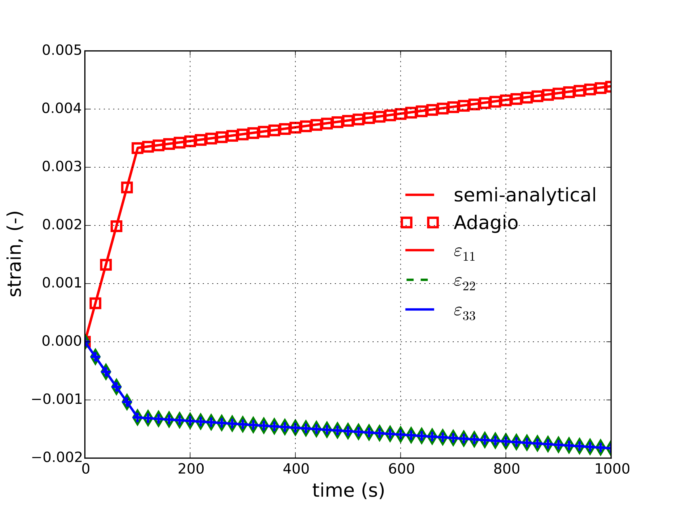
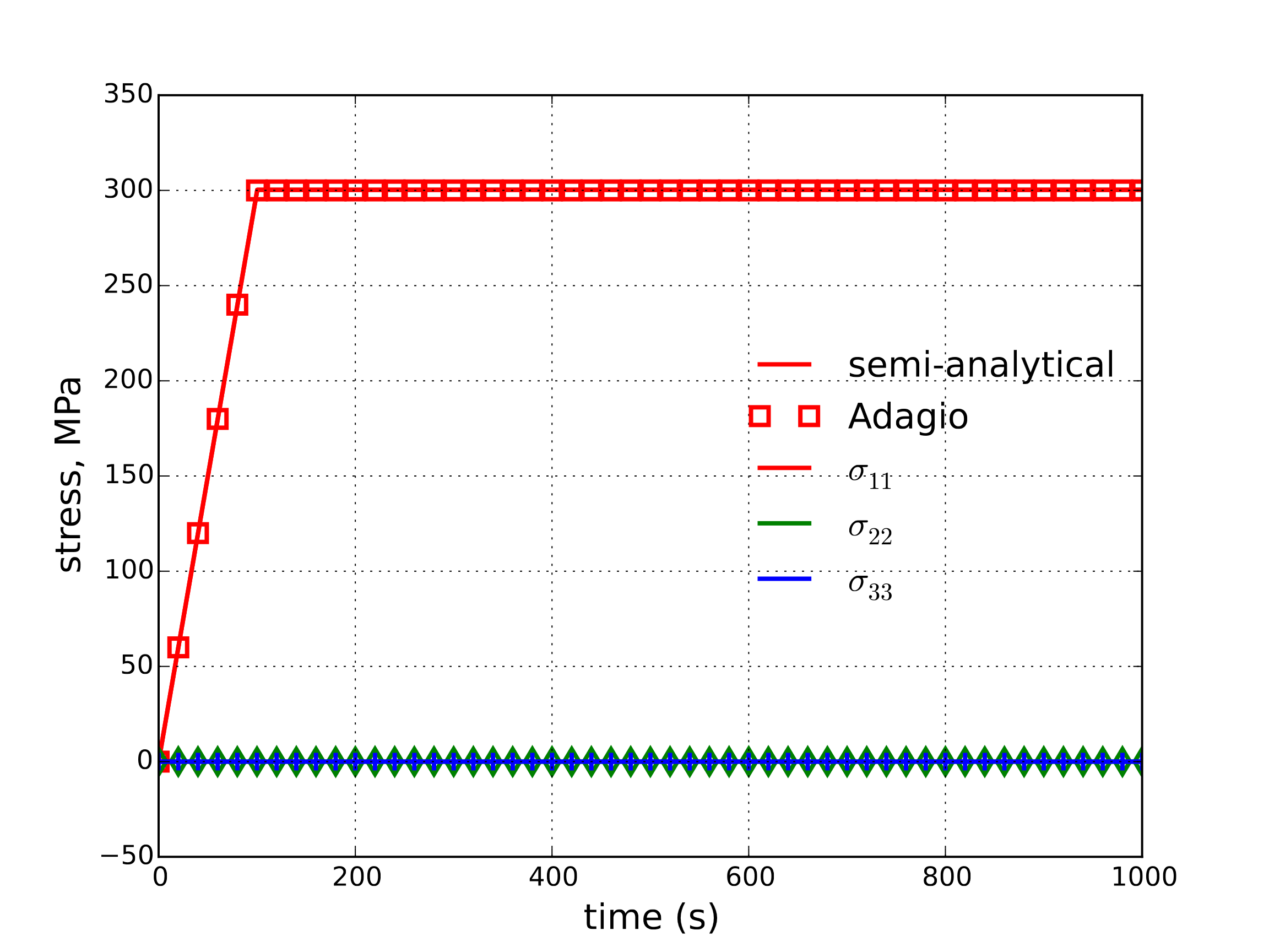
To consider the creep response, the model response is determined both numerically and semi-analytically. Through such a response, the stress tensor is \(\sigma_{ij}=\sigma\left(t\right)\delta_{i1}\delta_{j1}\) where \(\sigma\left(t\right)\) is a prescribed boundary condition. For this investigation, \(\sigma\left(t\right)\) ramps linearly from \(0\) to \(\sigma_{max}\) over the interval \(t=[0,100~\text{s}]\) and \(\sigma_{max}=300\) MPa. The stress is then held constant (\(\dot{\sigma}=0\)) for the next 900 s. Inverting the constitutive law (4.76) for the strain rate yields,

\[D_{ij}=\mathbb{S}_{ijkl}\dot{\sigma}_{kl}+D^{\text{c}}_{ij}.\]

Furthermore, given the stress tensor form above, the creep deformation rate is,

(4.77)\[D^{\text{c}}_{ij}=A\bar{\sigma}_{vM}^m\exp\left(\frac{-Q}{R\theta}\right)\left[\delta_{i1}\delta_{j1}-\frac{1}{2}\left(\delta_{i2}\delta_{j2}+\delta_{i3}\delta_{j3}\right)\right],\]

and

\[\mathbb{S}_{ijkl}\dot{\sigma}_{kl}=\dot{\sigma}\mathbb{S}_{ij11}.\]

The total deformation rate may then be determined and easily integrated to find an analytical response for the strain. To this end, both the semi-analytical and numerical strain and stress responses (as a function of time) are presented in Fig. 4.95(a) and Fig. 4.95(b), respectively.

Strain

Stress

Fig. 4.95 Semi-analytical and numerical results of (a) strain and (b) stress evolution during a creep test.

4.19.3.2. Stress Relaxation

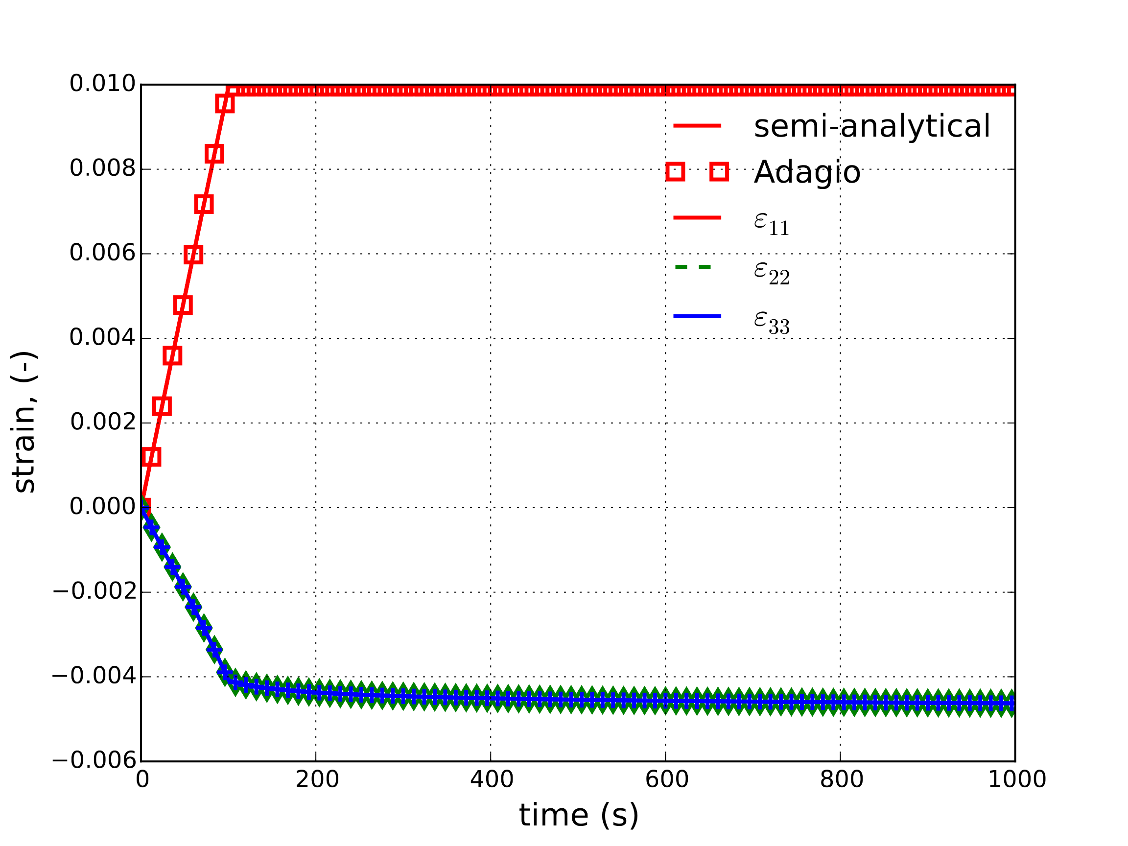
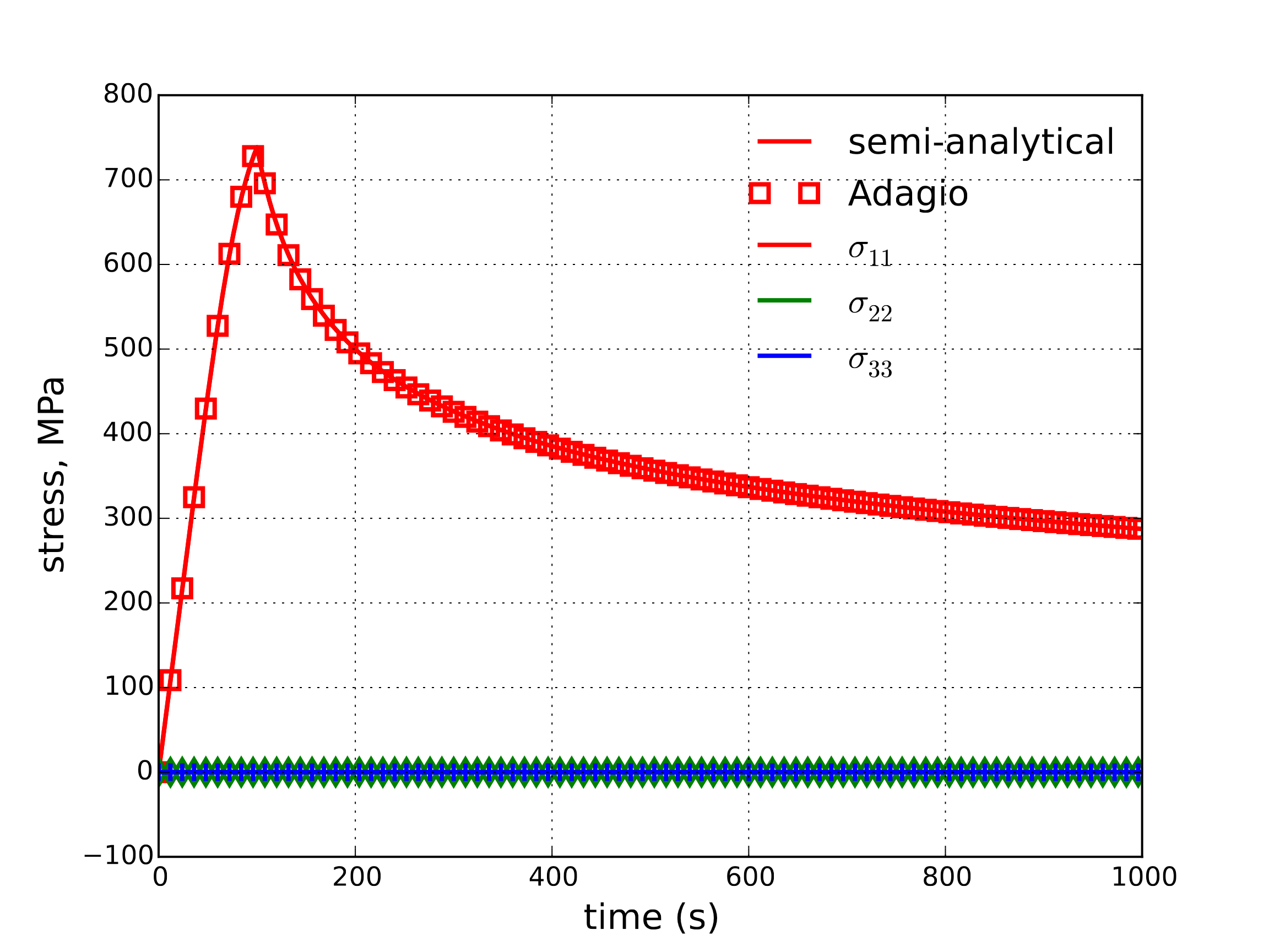
The stress relaxation response of the considered model is evaluated both numerically and semi-analytically. Specifically, a displacement controlled loading of \(u_1=\lambda\left(t\right)\) is investigated. The other displacement degrees of freedom are not constrained so that a uniaxial stress state results – \(\sigma_{ij}\left(t\right)=\sigma\left(t\right)\delta_{i1}\delta_{j1}\). The displacement is prescribed such that it scales linearly from \(u_1=0\) at \(t=0\) to \(u_1=.01\) at \(t=100\) s and then held fixed for 900 s. Initially the considered element is of unit length.

To determine the material response, it is noted that: (emph{i}) \(\sigma_{22}=\sigma_{33}=0\); (emph{ii}) \(D^{\text{e}}_{22}=D^{\text{e}}_{33}\) due to isotropy; and (emph{iii}) the creep deformation rate takes the form (4.77). With these observations, the elastic deformation rate in the direction of loading (\(D^{\text{e}}_{11}\)) becomes,

(4.78)\[D^{\text{e}}_{11}=\frac{\dot{\lambda}\left(t\right)}{1+\lambda\left(t\right)}-A\bar{\sigma}_{vM}^m\exp\left(\frac{-Q}{R\theta}\right).\]

Additionally, from (emph{i}) and (emph{ii}) above, it may be found that,

(4.79)\[D^{\text{e}}_{22}=D^{\text{e}}_{33}=-\nu D^{\text{e}}_{11},\]

leading to an equation for the stress in the direction of loading of,

\[\dot{\sigma}_{11}=\left(\mathbb{C}_{1111}-2\nu\mathbb{C}_{1122}\right)D^{\text{e}}_{11}.\]

Additionally, as \(D_{ij}=D^{\text{e}}_{ij}+D^{\text{c}}_{ij}\) the strains may easily integrated by using relations (4.77), (4.78), and (4.79). The resultant numerical and semi-analytical strain and stress responses are shown in Fig. 4.96(a) and Fig. 4.96(b), respectively.

Strain

Stress

Fig. 4.96 Semi-analytical and numerical results of the (a) strain and (b) stress evolution during a stress relaxation test.

4.19.4. User Guide

BEGIN PARAMETERS FOR MODEL POWER_LAW_CREEP
  #
  # Elastic constants
  #
  YOUNGS MODULUS = <real>
  POISSONS RATIO = <real>
  SHEAR MODULUS  = <real>
  BULK MODULUS   = <real>
  LAMBDA         = <real>
  TWO MU         = <real>
  #
  # Viscoplastic parameters
  #
  CREEP CONSTANT    = <real>
  CREEP EXPONENT    = <real>
  THERMAL CONSTANT  = <real>
  MAX SUBINCREMENTS = <integer> (100)
END [PARAMETERS FOR MODEL POWER_LAW_CREEP]

In the above command blocks:

• The creep constant, \(A\), in (4.75) is defined with the CREEP CONSTANT command line.

• The creep exponent, \(m\), in (4.75) is defined with the CREEP EXPONENT command line.

• The thermal constant, \(Q/R\) in (4.75) is defined with the THERMAL CONSTANT command line.

• Time step sub incrementation within the material model may be used to accurately calculate the true creep stress. The maximum sub-increments in a load step is defined with the MAX SUBINCREMENTS command line. The default is 100. A larger number of steps can potentially improve accuracy if a large amount of creep happens in a single step. A smaller number of steps can sometimes improve analysis speed.

Output variables available for this model are listed in Table 4.29.

Table 4.29 State Variables for POWER LAW CREEP Model

Name	Description
ECREEP	equivalent creep strain
SEQDOT	equivalent stress rate

---

[1]

J. Lemaitre and J.-L. Chaboche. Mechanics of Solid Materials. Cambridge University Press, 1990.

[2]

F.K.G. Odqvist. Mathematical theory of creep and creep rupture. Clarendon Press, Oxford, 1966.

[3] (1,2)

C.M. Stone. SANTOS – a two-dimensional finite element program for the quasistatic, large deformation, inelastic response of solids. Technical Report SAND90-0543, Sandia National Laboratories, Albuquerque, NM, 1996. \href http://infoserve.sandia.gov/sand_doc/1990/900543.pdfpdf.

[4]

W.M. Scherzinger and D.C. Hammerand. Testing of constitutive models in LAME. Technical Report SAND2007-5872, Sandia National Laboratories, Albuquerque, NM, September 2007. \href http://infoserve.sandia.gov/sand_doc/2007/075872.pdfpdf.