4.5. Neo-Hookean Model
4.5.1. Theory
The neo-Hookean model is a hyperelastic generalization of isotropic, small-strain linear elasticity. The stress-strain response for the neo-Hookean model may be determined from a free energy function - in this case the strain energy density, \(W\). The form of the strain energy density [[1]] is
where \(K\) and \(\mu\) are the bulk and shear moduli, respectively. The deformation measure is given by \(C_{ij}\), the components of the right Cauchy-Green tensor, where \(C_{ij} = F_{ki}F_{kj}\). The determinant of the deformation gradient is given by \(J\) and is a measure of the volumetric part of the deformation. \(\bar{C}_{ij}\) provides the isochoric part of the deformation and is given by
The second Piola-Kirchoff stress, with components \(S_{ij}\), may be determined by taking a derivative of the strain energy density and the Cauchy stress may be found by mapping from the second Piola-Kirchoff stress. The components of the Cauchy stress are
where \(B_{ij} = F_{ik}F_{jk}\), are the components of the left Cauchy-Green tensor and \(\delta_{ij}\) is the Kronecker delta.
Linearizing (4.10) we recover small strain linear elasticity
The neo-Hookean model is used for the recoverable (elastic) part for a number of inelastic, finite deformation constitutive models.
4.5.2. Implementation
As a hyperelastic model, the current state of the material may be determined by the total deformation. To this end we use the polar decomposition of the deformation gradient,
in which \(V_{ij}\) are the components of the left stretch tensor and \(R_{ij}\) is the corresponding rotation. Noting that,
and \(J=\det\left(V_{ij}\right)\), the Cauchy stress (via (4.10)) is found. The unrotated stress, \(T_{ij}\), which is needed for internal force calculations in Sierra/SM, is found using the transformation
4.5.3. Verification
It is possible to find closed form solutions for a number of loadings. Five problems are described here: uniaxial stress, pure shear strain, pure shear stress, uniaxial strain and simple shear. One set of material properties was used for all tests and they are given in Table 4.3. The elastic modulus and Poisson’s ratio are given in addition to the bulk and shear moduli.
\(K\) |
0.5 MPa |
\(\mu\) |
0.375 MPa |
\(E\) |
0.9 MPa |
\(\nu\) |
0.2 |
4.5.3.1. Uniaxial Stress
For uniaxial stress we will assume, without loss of generality, that \(\sigma_{11} \ne 0\). The deformation, in terms of the components of the left stretch tensor, for this stress state is
with all other components being zero.
The Cauchy stress is given by (4.10), however for simplicity we will use the Kirchhoff stress instead
where in what follows \(\tau_{11} = \tau\). With the lateral stresses being zero we have two equations
First, we solve for \(J\) by looking at the trace of the stress tensor. This gives us
Once we have \(J\) we can write \(\lambda_{2}^{2} = J/\lambda_{1}\) and solve for \(\lambda_{1}\) by looking at the deviatoric part of the Kirchhoff stress. For this we have
Rearranging we get a cubic equation for \(\lambda_{1}\)
A solution for this can be found with the following substitution
which gives a quadratic equation for \(x^{3}\)
The one meaningful solution to this polynomial is
with which we can substitute into (4.13) to get \(\lambda_{1}\). With \(J\) and \(\lambda_{1}\) we can solve for \(\lambda_{2}\). Note that in this solution the axial Kirchhoff stress, \(\tau\), is the independent variable.
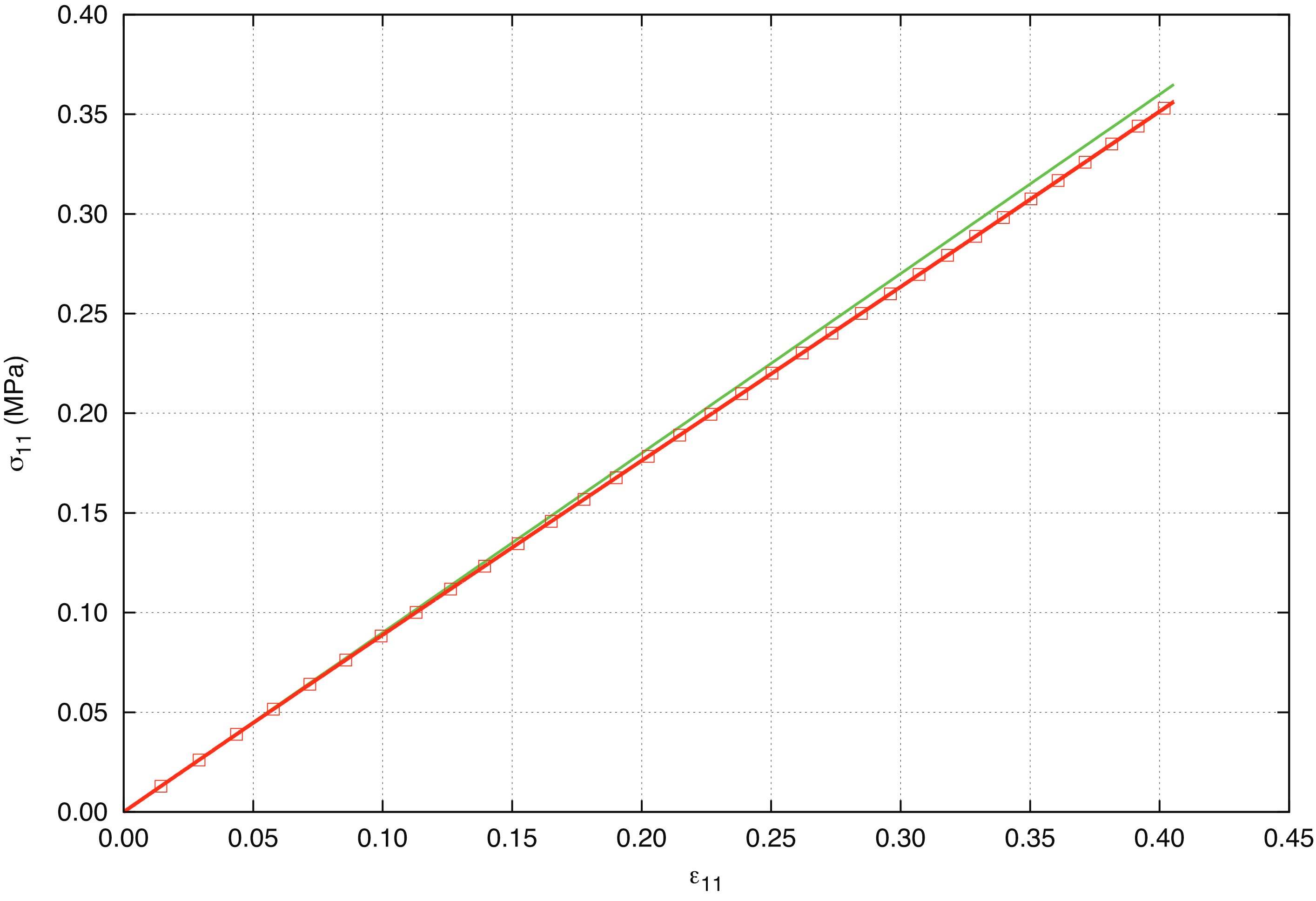 Axial stress
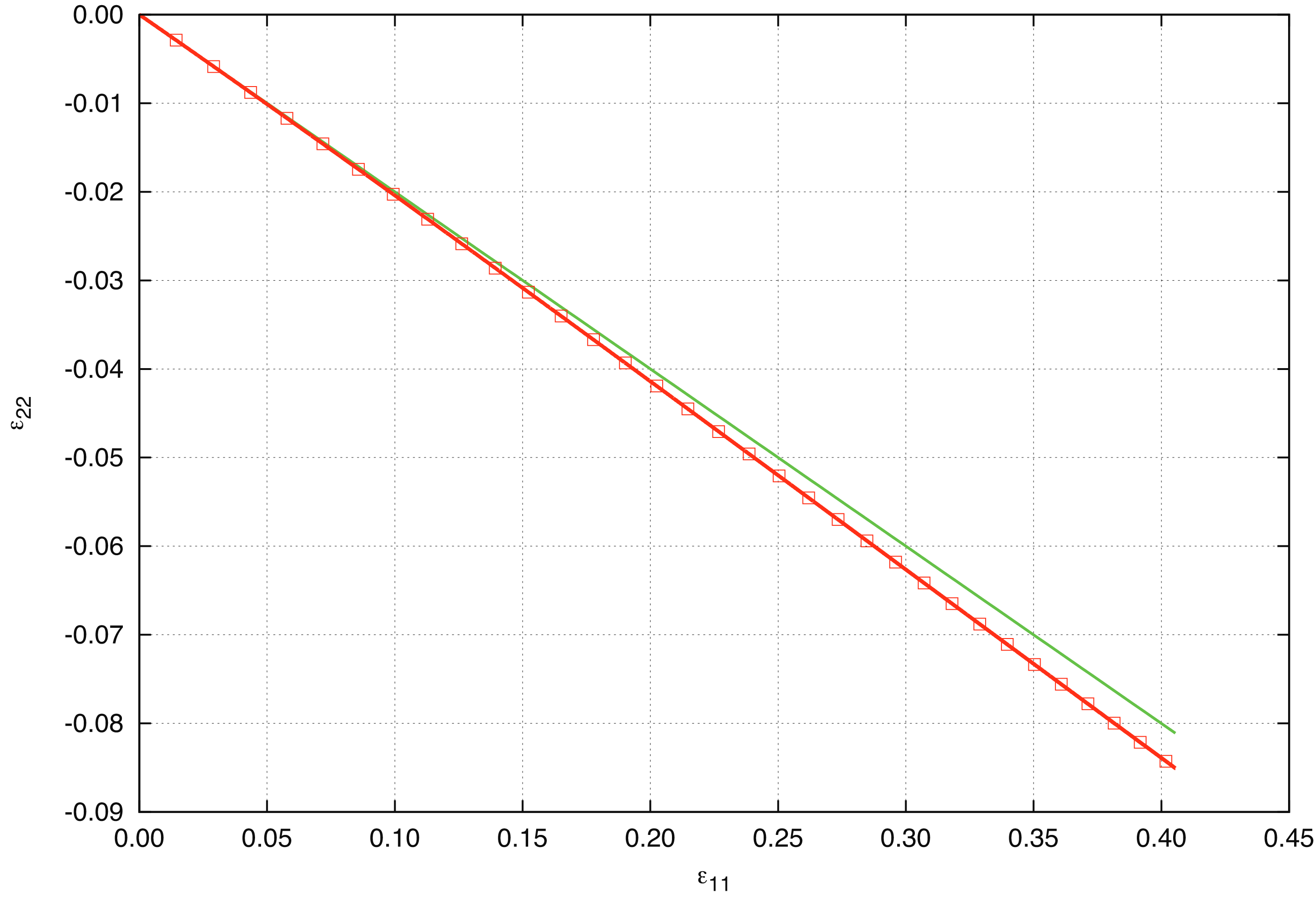 Lateral Strain
Fig. 4.8 Analytical and numerical results for the (a) uniaxial stress and (b) lateral strain. The green line gives the linear elastic response.
This solution is compared to the solution from a single element problem in Sierra/SM in Fig. 4.8(a) and Fig. 4.8(b). It should be noted that the response of the neo-Hookean model is slightly nonlinear. The linear elastic solution is given by the green line in each figure.
4.5.3.2. Pure Shear Strain
For pure shear strain the deformation gradient, which is symmetric, is
which gives no volume change, \(J=1\). Since there is no volume chance, the Kirchhoff stress is equal to the Cauchy stress: \({\boldsymbol\tau} = {\boldsymbol\sigma}\). Using (4.10), the non-zero stress components are
The results of a single element problem in Sierra/SM are compared with the analytical solution in Fig. 4.9. It is interesting to note that the normal stresses, \(\sigma_{11}\), \(\sigma_{22}\), and \(\sigma_{33}\) are not equal to zero. This is a much different result than what we get for the linear hypoelastic model.
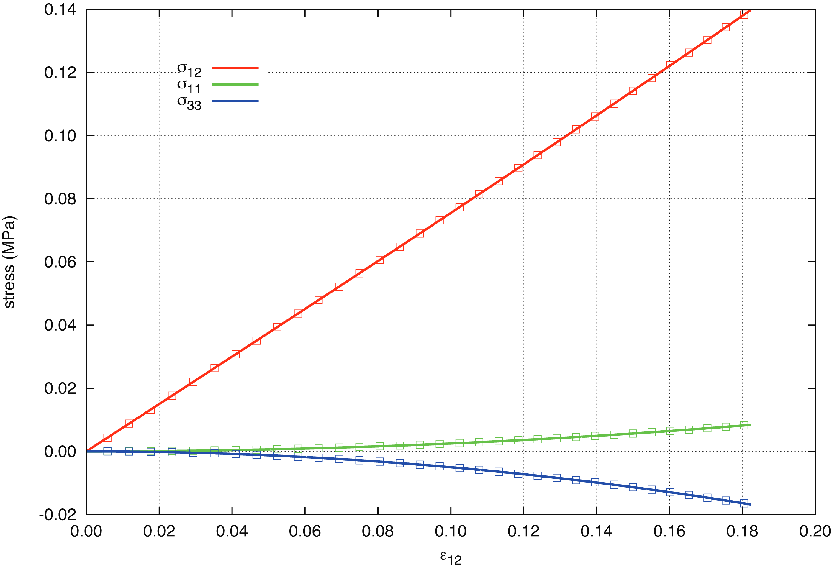
Fig. 4.9 Analytical and numerical results for the neo-Hookean model subjected to a pure shear strain. The solid lines are the analytical results and the boxes are results from Sierra/SM.
4.5.3.3. Pure Shear Stress
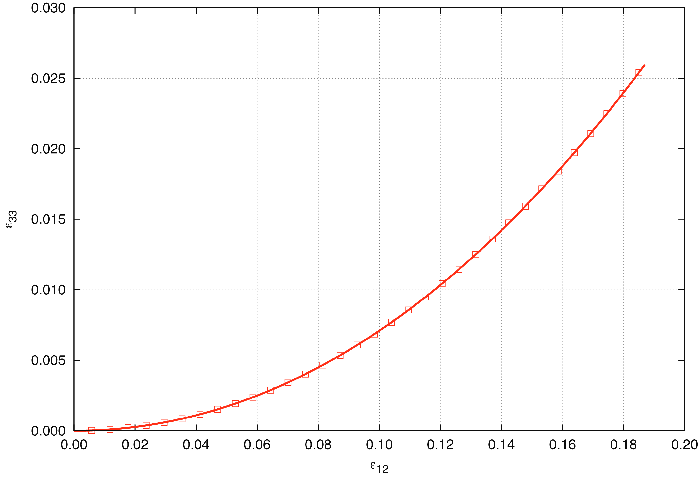
Fig. 4.10 Analytical and numerical results for the neo-Hookean model subjected to a pure shear stress. The curve gives the logarithmic strain component, \(\varepsilon_{33} = \frac{1}{2} \ln B\). The solid lines are the analytical results and the boxes are results from Sierra/SM.
Since pure shear strain did not result in a pure shear stress state, we do not expect a pure shear stress state to result in a pure shear strain state. For pure shear stress the only non-zero stress component is
and using (4.10) it can be shown that \(J=1\). The deformation, in terms of the left Cauchy-Green deformation tensor, is
The equation we need to solve for the deformation is \(\det{\bf B} = 1\). This gives us the cubic equation
This is a cubic equation of the same form as that in the uniaxial stress problem. We make the substitution
This gives us a quadratic equation in \(x^{3}\)
which has the solution
Substituting this solution into (4.14) gives \(B\).
The results of a single element problem in Sierra/SM are compared with the analytical solution in Fig. 4.10. Of interest here is the fact that the normal strains, \(\varepsilon_{11}\), \(\varepsilon_{22}\), and \(\varepsilon_{33}\) are not equal to zero. Again, this is a different result than what we get for the linear hypoelastic model.
4.5.3.4. Uniaxial Strain
First, utilizing a displacement condition corresponding to uniaxial strain results in a deformation gradient of the form,
By evaluating relation (4.10) with this deformation field produces stresses that may be written as
with the shear stress components equal to zero. Both the corresponding analytical and numerical solutions are presented in Fig. 4.11.
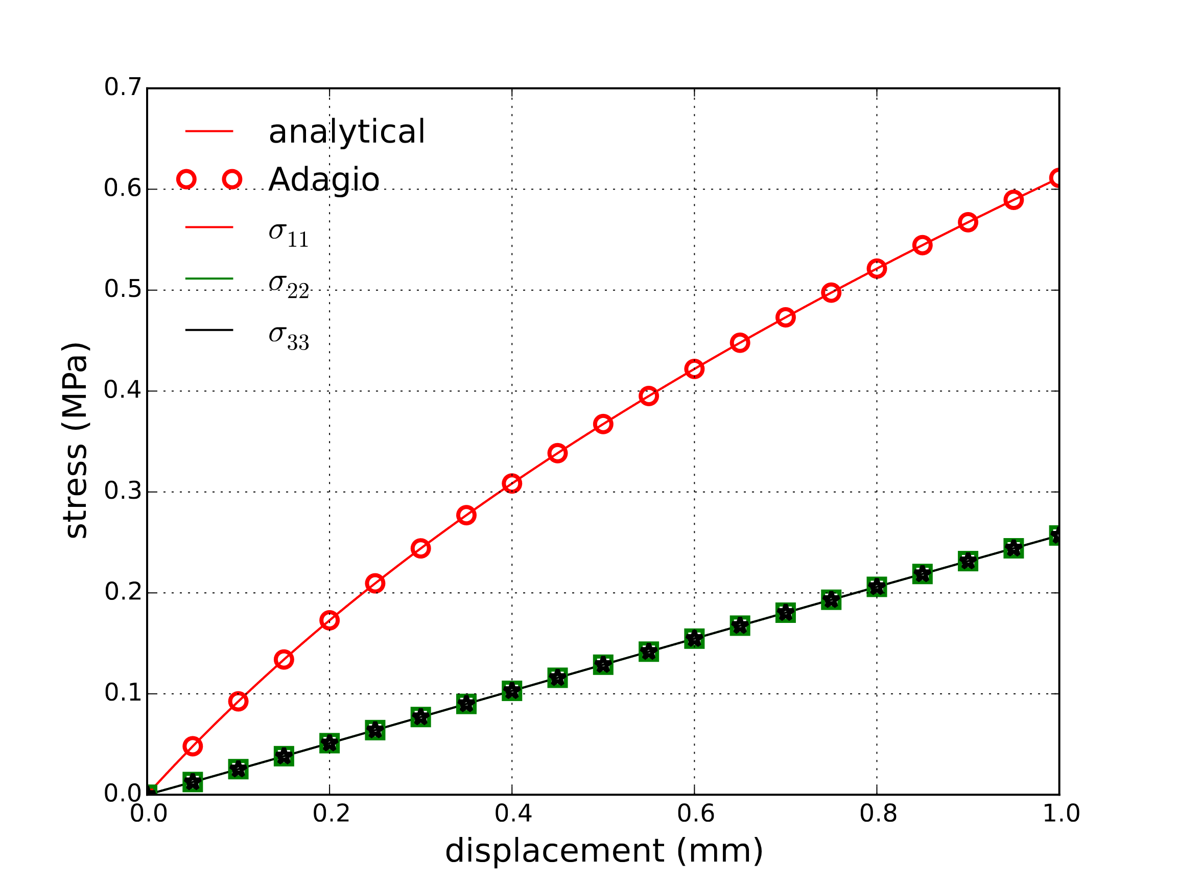
Fig. 4.11 Analytical and numerical results for the uniaxial stretch case.
4.5.3.5. Simple Shear
For the simple shear case, a deformation gradient of the form,
is assumed. Noting this is a volume preserving deformation (\(J=1\)) and again evaluating (4.10) produces stresses that may be written as,
Both the corresponding analytical and numerical solutions are presented in Fig. 4.12.
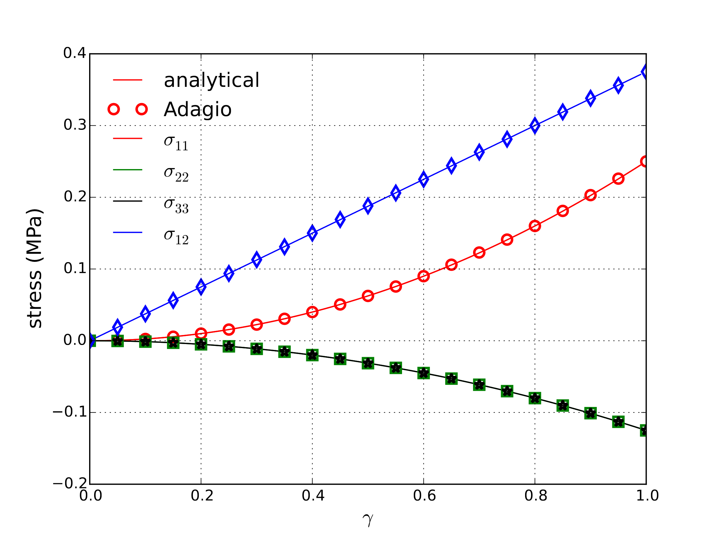
Fig. 4.12 Analytical and numerical results for the simple shear case.
4.5.4. User Guide
BEGIN PARAMETERS FOR MODEL NEO_HOOKEAN
  #
  # Elastic constants
  #
  YOUNGS MODULUS = <real>
  POISSONS RATIO = <real>
  SHEAR MODULUS  = <real>
  BULK MODULUS   = <real>
  LAMBDA         = <real>
  TWO MU         = <real>
END [PARAMETERS FOR MODEL NEO_HOOKEAN]
There are no output variables available for the neo-Hookean model.