3.4.4. Discrete system of equations

The full approximate pressure projection scheme for non-uniform density is now written as

(3.793) $\eta M_{L}^k \Delta \hat u_i + C_{L}( \dot m^k)\Delta \hat u_i - T_{Lj}\Delta \hat u_i =-r_i,$

(3.794) $-L_{{\tau_1}{L}}\Delta p^{n+{1\over2}}= -D_L(\hat u_i) - L_{{\tau_{1}}}p^{k}+(L_2-D \tilde \tau_2 G)_Lp^k+b,$

(3.795) $u_{Li}^{n+1} = \hat u_{Li} - \tilde \tau G_{Li}\Delta p^{n+{1\over2}}.$

The variable $-r_i$ is the residual that includes body source terms, pressure gradient, the non-symmetric part of the viscous stress term, $T^{ns}_{Li} u_j^k$ , parts of the time term and the left-hand side set of operators acting on the $u_i^k$ state,

(3.796) $-ri = -\eta M_{L}^k u_i^k - C_{L}( \dot m^k) u_i^k + T_{Lj}\Delta u_i^k +T^{ns}_{Li} u^{k}_j +S_{Li}-(1-\eta)M_L(\dot{\rho u_i^n})-G_{Li}p^{n-{1\over2}}.$

The mass matrix, $M_{L}^k \Delta \hat u_i$ , is defined by

(3.797) $M_{L}^k \Delta \hat u_i= \sum_{\alpha ' \in {\mathcal B}_L} \left(\sum_{K \in {\mathcal N}} N_K ({\bf x}_{\alpha'}) {{\rho_K^{k }} \over {\Delta t}}\right)\left(\sum_{K \in {\mathcal N}} N_K ({\bf x}_{\alpha '}) \Delta \hat u_{Ki}\right) dV_{\alpha '} .$

The shape function above, $N_K({\bf x}_{\alpha'})$ , is frequently evaluated at ${\bf x}_{\mathcal N}$ , the coordinates of the vertex associated with the transport equation, i.e., the case where a lumped mass matrix is used.

For simplicity, the central difference operator is provided in $C_{Li}\Delta \hat u_i$ as

(3.798) $C_{L} \Delta \hat u_i= \sum_{\alpha \in {\mathcal B}_L}m^k_{\alpha}\left(\sum_{K \in {\mathcal N}} N_K ({\bf x}_\alpha) \Delta \hat u_{Ki}\right).$

In the preceding equation, the mass flow rate has been linearized within the iteration step and may or may not include the explicit stabilization terms. Moreover, the shape function operator, $N_K({\bf x}_{\alpha})$ , may be evaluated at the edge midpoints to retain the skew symmetric aspect of the operator $C_L$ . By default, this term is evaluated at the subcontrol surface integration points, which retains the CVFEM canonical 27-point stencil.

The symmetric part of the stress tensor is given by

(3.799) $T_{Lj} \hat u_i = \sum_{\alpha \in {\mathcal B}_L} \left(\sum_{K \in {\mathcal N}} N_K ({\bf x}_\alpha) \mu_K\right) \left( \sum_{K \in {\mathcal N}} {{dN_K ({\bf x}_\alpha)} \over {dx_j}} \hat u_{Ki}\right) n_j({\bf x}_{\alpha}) \Delta A_{\alpha} ,$

while the non-symmetric stress tensor is given by

(3.800) $T^{ns}_{Li} u^{k}_j = \sum_{\alpha \in {\mathcal B}_L} \left(\sum_{K \in {\mathcal N}} N_K ({\bf x}_\alpha) \mu_K\right) \left(\sum_{K \in {\mathcal N}} {{dN_K ({\bf x}_\alpha)} \over {dx_i}} u^{k}_{Kj}\right) n_j({\bf x}_{\alpha}) \Delta A_{\alpha} - { {2} \over {3}} \sum_{\alpha \in {\mathcal B}_L} \left(\sum_{K \in {\mathcal N}} N_K ({\bf x}_\alpha) \mu_K\right)\left(\sum_{K \in {\mathcal N}} {{dN_K ({\bf x}_\alpha)} \over {dx_p}} u^{k}_{Kp}\right) \delta_{ip}n_p({\bf x}_{\alpha}) \Delta A_{\alpha} .$

Note that the nodal pressure gradient at node $L$ for control volume $L$ for direction $i$ is defined by (3.754). The operator, $S_{Li}$ , contains the gravitational term as well as the [potentially] subtracted out hydrostatic term,

(3.801) $S_{Li} = \sum_{\alpha' \in {\mathcal B}_L} \left(\sum_{K \in {\mathcal N}} N_K ({\bf x}_{\alpha'}) (\rho^k_K-\rho^{ref})\right)g_idV_{\alpha'} .$

The old time term contribution, $M_L(\dot{\rho u_i}^n)$ , is defined by

(3.802) $M_{L}(\dot{\rho u_i}^n) = \sum_{\alpha ' \in {\mathcal B}_L} \left(\sum_{K \in {\mathcal N}} N_K ({\bf x}_{\alpha'}) \dot{ {\rho_K u_{Ki}}^n}\right)dV_{\alpha '} .$

Again, $\alpha' \in {\mathcal B}_L$ is the set of all subcontrol volume integration points for control volume $L$ , $\alpha' \in {\mathcal B}_L$ is the set of all subcontrol surface integration points for control volume $L$ , and $K \in {\mathcal N}$ is the set of all nodes within the element.

3.4.4.1. Predictor

In general, there are a number of predictors that are supported. The easiest predictor is a simple predictor in which the old value is mapped into the current iterate. Predictors that incorporate old time derivatives include the forward Euler and Adams-Bashforth methods, e.g.,

(3.803) $\phi^{k+1} = \phi^n ,$

(3.804) $= \phi^n + \Delta t \dot \phi^n ,$

(3.805) $= \phi^n + {{\Delta t^n} \over {2}} (( 2 + { {\Delta t^n} \over {\Delta t^{n-1}} } ) \dot \phi^n - { {\Delta t^ n} \over {\Delta t^{n-1}} } \dot \phi^{n-1} ).$

3.4.4.1.1. Upwind Interpolation for Convection

We currently support several upwind interpolations for convection. The upwind methods are blended with a centered scheme that becomes dominant below a specified cell-Peclet number.

3.4.4.2. First Order Upwind

The first scheme is a simple first-order scheme that considers the two nodes adjacent to a control volume face and extrapolates from the node in the upwind direction.

(3.806) $\dot{m} \overline{\phi}_{upw} = {1 \over 2} \left( \dot{m} + \left| \dot{m} \right| \right) \phi_L + {1 \over 2} \left( \dot{m} - \left| \dot{m} \right| \right) \phi_R$

The convention is that flow leaves the control volume to the left (L) and enters the control volume to the right (R). If the mass flow rate at the face is negative in value, then the node to the right will be selected.

3.4.4.3. Blending Function

The user specified upwind factor controls the blending between the pure upwind operator and a blended user-chosen upwind/central operator.

(3.807) $\dot{m} \overline{\phi} = \eta \dot{m}\overline{\phi}_{upw} + (1-\eta)\left( \chi \dot{m} \overline{\phi}_{upw^{sp}} + \left( 1 - \chi \right) \dot{m} \overline{\phi}_{cen}\right) ,$

where $\eta$ is the user specified first order upwind factor and $\overline{\phi}_{upw^{sp}}$ represents the user specified upwind operator, e.g., MUSCL, modified skew upwind, and even pure upwind.

The centered average of $\phi$ is computed from the shape functions, so it is based on all nodes in an element. The shape functions are evaluated at the sub-face centroid. The cell-Peclet number, ${\rm Pe}_{\Delta x}$ , is used in the blending function (see Figure 3.29)

(3.808) $\chi = {{ \left({\zeta \rm Pe_{\Delta x}}\right)^2} \over { 5 + {\left({\zeta \rm Pe_{\Delta x}}\right)^2}}} .$

The hybrid upwind factor, $\zeta$ , allows one to modify the functional blending function; values of unity result in the normal blending function response in Figure 3.29; values of zero yield a pure central operator, i.e., blending function = 0.0; values $>>$ 1 result in a blending function value of unity, i.e., pure upwind. The constant $A$ is implemented as above with a value of 5. This value can not be changed via the input file.

The cell-Peclet number is computed for each sub-face in the element from the two adjacent left (L) and right (R) nodes.

(3.809) ${\rm Pe}_{\Delta x} = {{{1 \over 2} \left( u_{R,i} + u_{L,i} \right) \left( x_{R,i} - x_{L,i} \right) } \over \nu }$

A dot-product is implied by repeated indices.

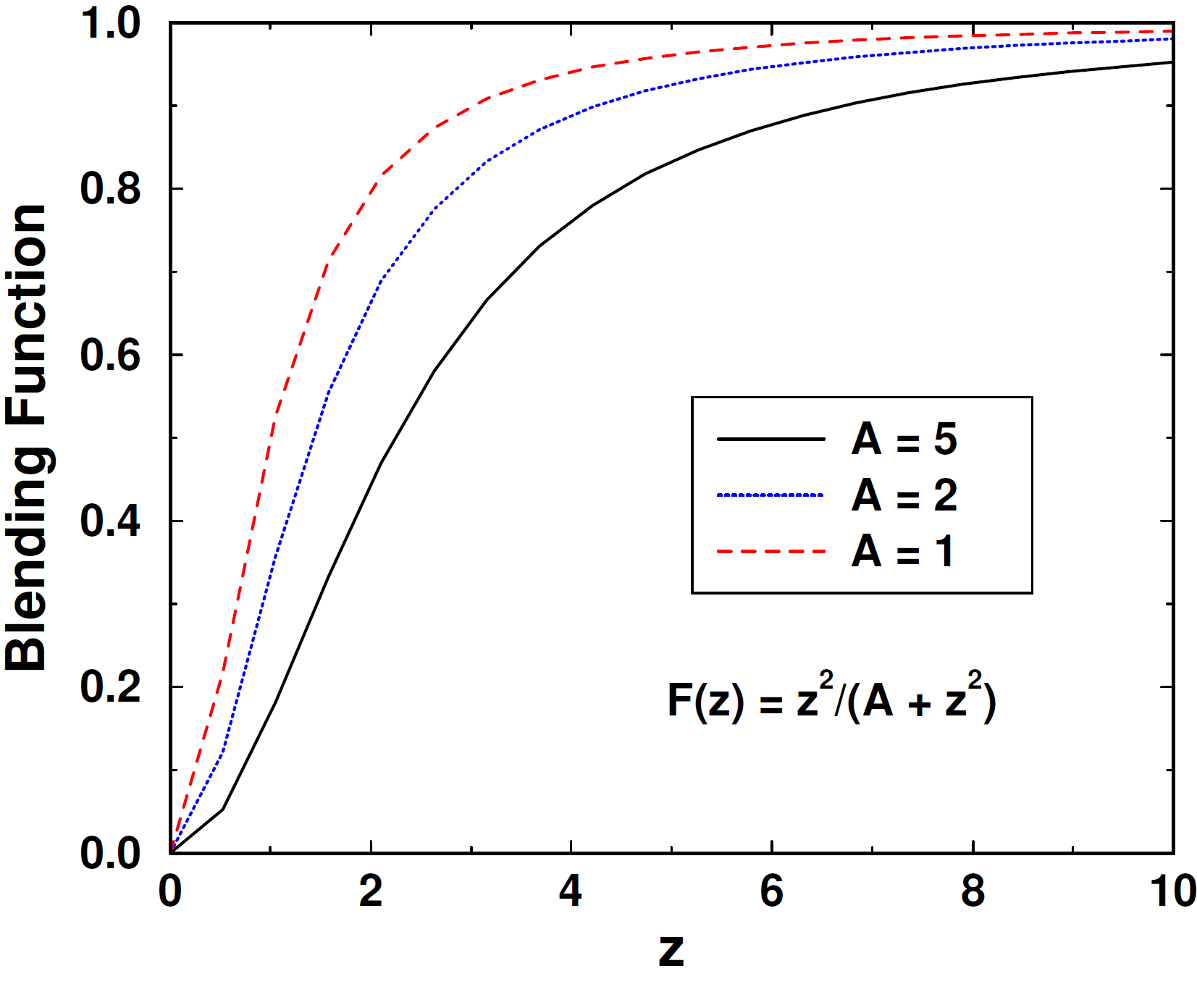
Fig. 3.29 Cell-Peclet number blending function.

3.4.4.4. Modified Linear Profile Skew Upwind

Modified linear profile skew upwinding is a simplification to the skew upwinding approach in the FIELDS scheme [150, 151]. We omit the physical advection correction terms. Integration point values at control volume subfaces are interpolated from upwind intersection points on the element face. In the original skew upwind scheme, the intersection point could either be interior subface or element faces. The interpolation coefficients were computed by inverting a matrix relation between integration point values and nodal values. The linear profile skew upwinding does not use interior subface intersections – only element face intersections. The modified scheme throws out nodes on an element face that are downwind of an interior subface as shown in Figure 3.30.

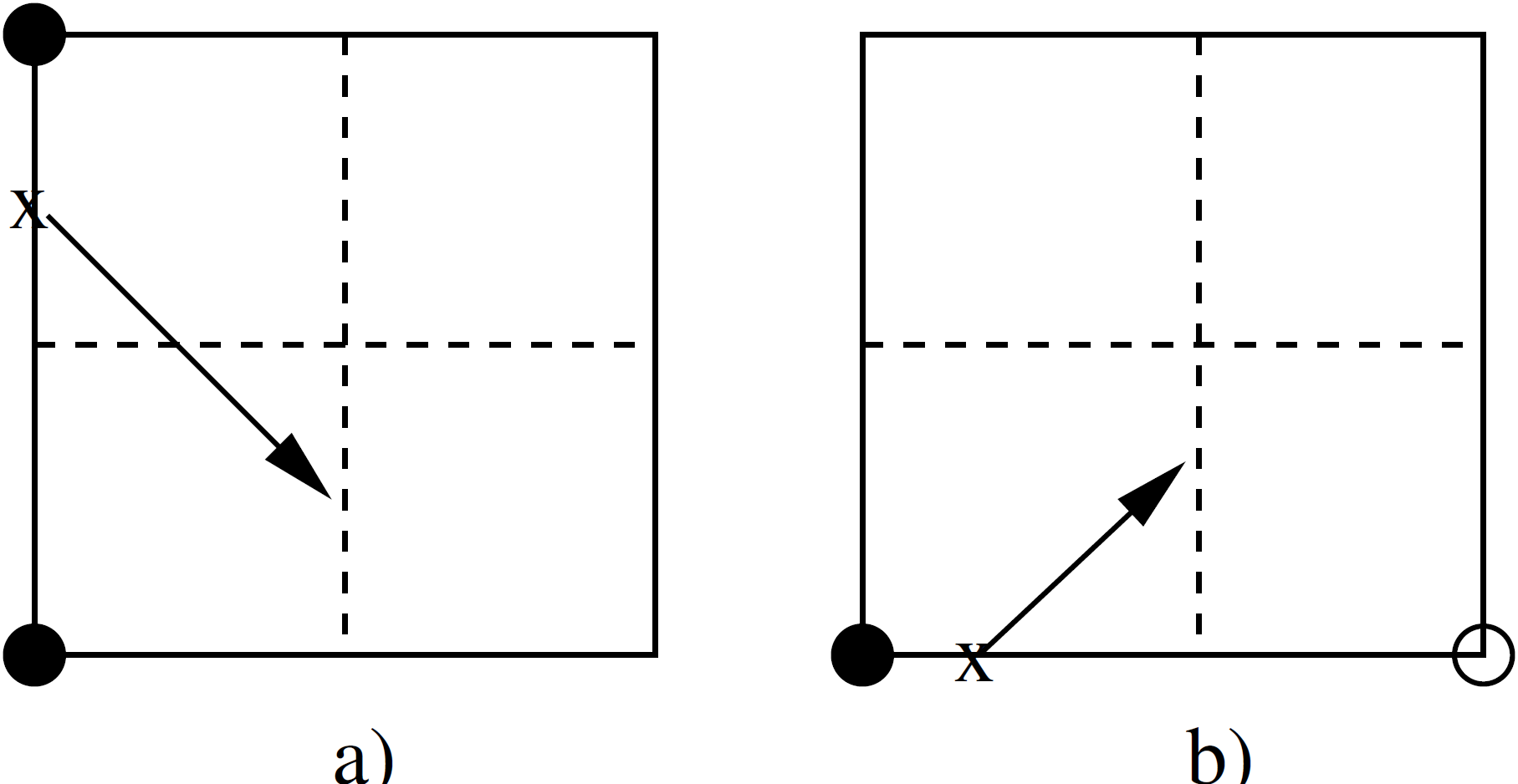
Fig. 3.30 Linear profile skew upwind scheme: a) all nodes on the intersected element face are upwind of the subface, b) omit nodes on intersected element face that are downwind of the subface.

3.4.4.5. MUSCL

The MUSCL approach (see Chap. 21 of Hirsch [230]) for higher order upwinding is adapted to unstructured meshes. The upwind interpolation is constructed along each edge of an element. The interpolation makes use of the two end nodes of the edge and the centered gradient constructed at the two end nodes. The MUSCL approach constructs an interpolation in one dimension from four (or more) uniformly distributed nodal values. The two edge nodes are $\phi_{i}$ and $\phi_{i+1}$ . The two other nodal values, $\phi_{i-1}$ and $\phi_{i+2}$ , are interpolated from the unstructured mesh using the nodal gradient information.

The MUSCL scheme constructs left and right interpolants at the subface of the control volume. Without the limiter functions, the interpolation is

(3.810) $\phi_{i+1/2}^L = \phi_{i \phantom{+1}} + {1 \over 4} \left[ \left( 1 - \kappa \right) \left( \phi_{i} - \phi_{i-1} \right) + \left( 1 + \kappa \right) \left( \phi_{i+1} - \phi_{i} \right) \right] ,$

(3.811) $\phi_{i+1/2}^R = \phi_{i+1} - {1 \over 4} \left[ \left( 1 + \kappa \right) \left( \phi_{i+1} - \phi_{i} \right) + \left( 1 - \kappa \right) \left( \phi_{i+2} - \phi_{i+1} \right) \right] ,$

where the $(i+1/2)$ location is between node $i$ and node $i+1$ . On a uniform mesh, $\kappa = 1/3$ gives a third-order scheme. A second-order upwind scheme is recovered with $\kappa = -1$ and a centered scheme is recovered with $\kappa = 1$ .

Limiter functions are introduced to prevent numerical oscillations from occurring.

(3.812) $\tilde{\phi}_{i+1/2}^L = \phi_{i \phantom{+1}} + {1 \over 4} \left[ \left( 1 - \kappa \right) \Phi \left( {1 \over {r_L}} \right) \left( \phi_{i} - \phi_{i-1} \right) + \left( 1 + \kappa \right) \Phi \left( r_L \right) \left( \phi_{i+1} - \phi_{i} \right) \right] ,$

(3.813) $\tilde{\phi}_{i+1/2}^R = \phi_{i+1} - {1 \over 4} \left[ \left( 1 + \kappa \right) \Phi \left( r_R \right) \left( \phi_{i+1} - \phi_{i} \right) + \left( 1 - \kappa \right) \Phi \left( {1 \over {r_R}} \right) \left( \phi_{i+2} - \phi_{i+1} \right) \right] ,$

where

(3.814) $r^L = {{\phi_{i} - \phi_{i-1}} \over {\phi_{i+1} - \phi_{i}}} ,$

(3.815) $r^R = {{\phi_{i+2} - \phi_{i+1}} \over {\phi_{i+1} - \phi_{i}}} .$

The limiters are selected to be symmetric such that

(3.816) $\Phi \left( r \right) = r \Phi \left( {1 \over r} \right) .$

The limited interpolation functions are

(3.817) $\tilde{\phi}_{i+1/2}^L = \phi_{i} + {1 \over 2} \Phi \left( r^L \right) \left( \phi_{i+1} - \phi_{i} \right) ,$

(3.818) $\tilde{\phi}_{i+1/2}^R = \phi_{i+1} - {1 \over 2} \Phi \left( r^R \right) \left( \phi_{i+1} - \phi_{i} \right) .$

The interpolation for the points off the element edge is

(3.819) $\left( \phi_{i} - \phi_{i-1} \right) = 2 \nabla \phi_{i} \Delta x_{i+1/2} - \left( \phi_{i+1} - \phi_{i} \right) ,$

(3.820) $\left( \phi_{i+2} - \phi_{i+1} \right) = 2 \nabla \phi_{i+1} \Delta x_{i+1/2} - \left( \phi_{i+1} - \phi_{i} \right) ,$

where $\Delta x_{i+1/2} = x_{i+1} - x_{i}$ is the distance vector along the element edge. Symmetric limiter functions are:

(3.821) ${\rm Van Leer:} \quad \quad \Phi(r) = {{r + \left| r \right|} \over {1 + \left| r \right| }} ,$

(3.822) ${\rm Van Albada:} \quad \quad \Phi(r) = {{r + r^2 } \over {1 + r^2}} ,$

(3.823) ${\rm superbee:} \quad \quad \Phi(r) = \max(0, \min(2r,1), \min(r,2)) .$

3.4.4.6. Convection at an Inflow and Outflow Boundary

At an open boundary, the first-order and LPS upwind schemes only make use of information on the boundary.

For the MUSCL scheme with the flow leaving the domain at node $i$ , the usual flux limiters are not used. The slopes are compared between $(\phi_i - \phi_{i-1})$ and $(\phi_{i-1} - \phi_{i-2})$ . If the slopes are the same sign, the unlimited second order upwinding is used. If the slopes are different, then a local interpolation is used. Estimate the slope $(\phi_{i-1} - \phi_{i-2}) = 2 \Delta x \nabla \phi_2 - (\phi_i - \phi_{i-1})$ , where $\Delta x_{i} = x_{i} - x_{i-1}$ is the distance vector along the element edge. For slopes of the same sign, use a second-order scheme,

(3.824) $\tilde{\phi}_{i}^L = \phi_{i} + {1 \over 2} \left( \nabla \phi_{i-1} \Delta x_i - \left( \phi_i - \phi_{i-1} \right) \right) , , , ,$

else, use a first-order scheme,

(3.825) $\tilde{\phi}_{i}^L = \phi_{i} - {1 \over 2} \left[ \left( \phi_i - \phi_{i-1} \right) \right] .$

The boundary is the left (L) side. If the flow enters the domain, then use the local value of $\phi_i$ .

3.4.4.7. Nonlinear stabilization operator

The “nonlinear stability operator” (NSO) in Fuego is an artificial viscosity method where the added diffusivity is based on a scaled, pointwise evaluated residual. For a dual volume ( $\Omega_n$ ), associated with a node $n$ , the weak form of the NSO for a scalar variable $q$ is

(3.826) $\int_{\partial \Omega_n} \nu(R) \left(\partial_{x^i} q\right) \, g^{ij} \, {\rm d}S_j, \mbox{ where } g^{ij} = \frac{\partial x^i}{\partial \xi^k} \frac{\partial x^j}{\partial \xi^k}.$

where $\nu$ depends on the evaluation of a local residual $R$ and the gradient of $q$ as

(3.827) $\nu = \sqrt{ \frac{R^2} {\frac {\partial q}{\partial x^i} g^{ij} \frac{\partial q}{\partial x^j}} }.$

The local residual can be taken, similar to Shakib:cite:Shakib:1991 but in an incompressible context, as the full residual of the PDE. For a conserved scalar,:math:q, with diffusivity $\Gamma$ , $R$ would be

(3.828) $R = \left[\left(\operatorname{Time}\right)_\rho + \left(\operatorname{Adv.}\right)_{\rho \mathbf{u}} - \left(\operatorname{Diff.}\right)_{\rho \Gamma}\right]q,$

with discrete operators representing the individual terms of the advection-diffusion equation. For an equation with a source term, it would also need appear in the local residual calculation. Another possibility for choosing $R$ would be based on the error of performing the chain-rule on the advection operator.

(3.829) $R = \tilde{G}_i\left(\rho u^i q\right) - \left[\tilde{I}\left(\rho u^i \right) \tilde{G}_i q + \left(\tilde{I}q\right) G_i \left(\rho u^i\right) \right]$

where $\tilde{G}$ and $\tilde{I}$ represent interpolation and gradients evaluated at an integration point. Both options are available in Fuego.

The NSO computed from such residuals can add an unnecessarily large amount of dissipation in some cases. For this reason, we limit the NSO coefficient to the upwind value as

(3.830) $\nu = \operatorname{min}\left(\nu(R), \frac{1}{10} \left(\rho u\right)^i g_{ij} \left(\rho u \right)^j \right).$

where $g_{ij} = \left[g^{ij}\right]^{-1}$ . Additionally, as it’s based on the mesh discretization error, the NSO coefficient tends to vary strongly on short length scales. For numerical robustness, we average the NSO viscosity over control volumes, and then interpolate back to the subcontrol surfaces to evaluate the diffusion term; that is,

(3.831) $\overline{\nu}_{\rm ip} = \tilde{I} \, \frac{\overline{\nu \| g^{ij} \|}}{\| g^{ij} \|}.$

This operation effectively smooths the NSO viscosity over a patch of elements. The nonlinear stabilization viscosity is not included at the boundaries.

3.4.4.7.1. Variable Density

The discretization of the time derivative requires special attention for variable density flows. The density time-derivative in the continuity equation must be predicted in a continuous manner. The density at the new time level in the convection terms and the transport equation time terms must also be predicted.

The transport equations are solved in conservative form, so density appears in the time derivative. With a segregated solution strategy, the density at the new time level is not available until the transport equations have been solved once. A density predictor is required. A generic time term is written as

(3.832) ${{\partial \rho \phi} \over {\partial t}} \approx { { \rho^{n+1} \phi^{n+1} - \rho^{n} \phi^{n} } \over { \Delta t } } \approx \rho^{n} { { \phi^{n+1} - \phi^{n} } \over { \Delta t } } + \phi^{n+1} { { \rho^{\ast} - \rho^{n} } \over { \Delta t } }$

There are two approaches to estimating the new density. The simplest approach is to use the most recent value. The other approach is to use a density predictor. The predicted value of density at the new time level, $\rho^{\ast}$ , is computed from the old density and the current density time derivative. Introduce the nodal variable $\Upsilon$ for the discrete density time-derivative such that

(3.833) $\Upsilon^{\ast} = { { \rho^{\ast} - \rho^{n} } \over { \Delta t } }$

(3.834) $\rho^{\ast} = \rho^{n} + { \Delta t } \Upsilon^{\ast}$

The density derivative, $\Upsilon^{\ast}$ , is always updated at the bottom of the transport equation loop after a new set of temperatures and mass fractions is available. The two approaches are different for the first nonlinear sub-iteration within a time step, but yield equivalent values upon subsequent sub-iterations. The new density is also computed at the bottom of the equation loop. This value is ignored upon subsequent sub-iterations if using the density predictor. But, this new density value will get copied to the old time level when the time step is advanced. It is important to note that this new “old” velocity is not consistent with the density that was used in the old transport equations, but it seems critical to the success of this approach to do so.

For the first nonlinear iteration within a time step, the effect of the density at the new time level is predicted by carrying forward the best approximation of the density time-derivative from the last time step. The continuity equation is implemented as

(3.835) $\int \Upsilon^{\ast} dV + \int \rho^\ast \overline{u_i}^{n+1} n_i dS = 0 ,$

where the density time-derivative is the most recent value and the density in the convection is estimated in the same manner as the transport equations. The density time-derivative, $\Upsilon$ , must be stored as a persistent nodal variable in order to have a good estimate for the continuity equation from step to step.

3.4.4.7.2. Open Boundary Conditions

Open boundary conditions are used for boundaries where the flow can go either in or out. The direction of the flow is determined by the local force balance. In this documentation, the open boundary condition is also referred to as the outflow boundary condition. There are two parts to the outflow boundary condition. The first part concerns computing a velocity field that satisfies continuity. The second part concerns selecting the proper convected scalar value depending if the flow is in or out of the domain. Control volume balances are implemented at open boundaries for continuity, momentum, and the other transport equations.

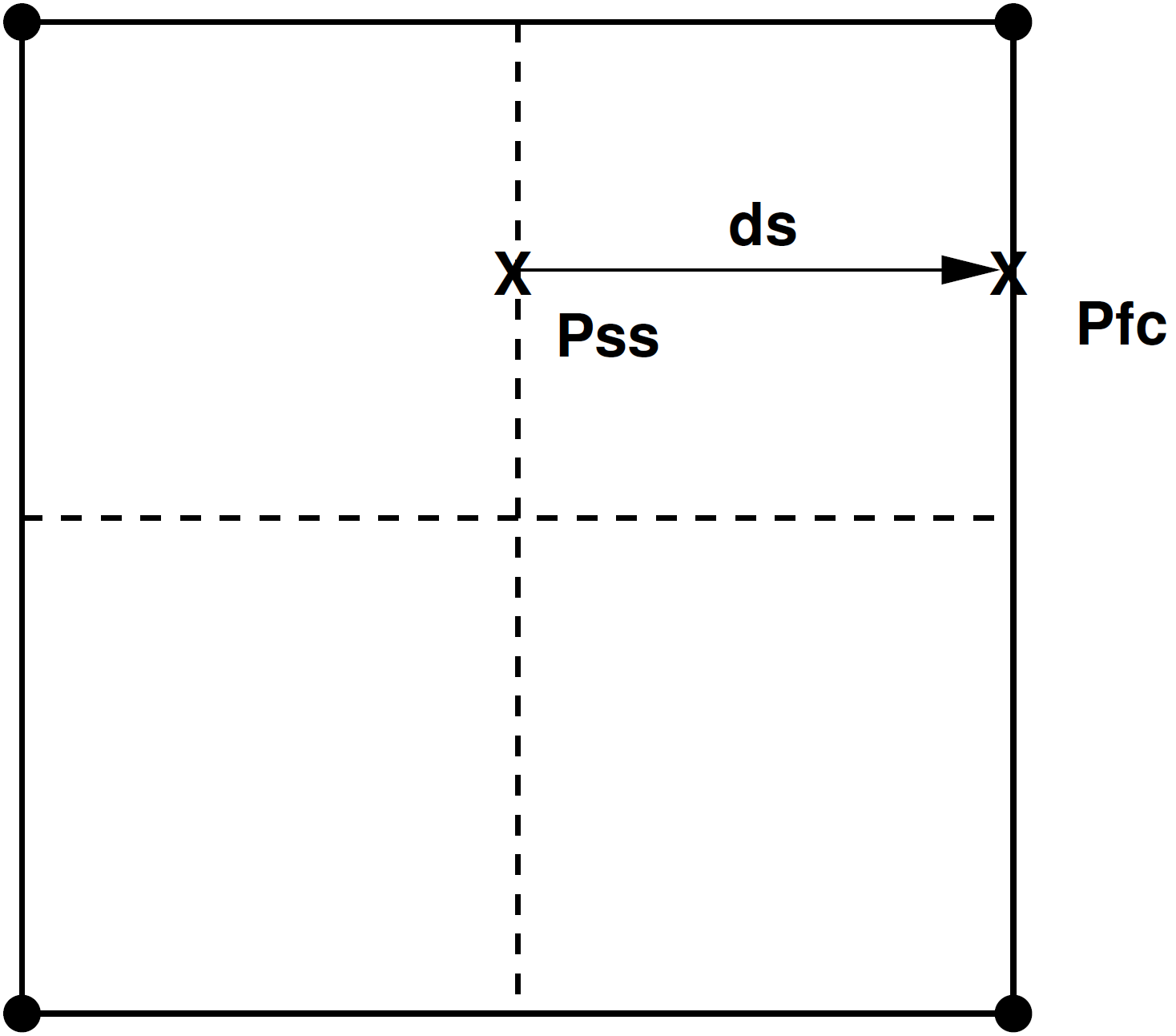
Fig. 3.31 Boundary mass flux integration locations.

A fixed pressure value is specified for the continuity and momentum equations. The nodal values of pressure on the boundary are allowed to float. A mass flux condition is formulated at the boundary in order to drive the boundary pressures towards the specified boundary pressure and to provide a boundary mass flow rate for the other transport equations. The form of the boundary mass flux is similar to the pressure-stabilized interior mass fluxes (see section Flow Solver). The equation for the mass flux at a boundary face, shown in Figure 3.31, is

(3.836) $\dot{m}_{\rm bc} = \rho \overline{u}_i^{n+1} n_i {\rm d}S$

and the interpolation formula for a single velocity component is

(3.837) $\overline{u}^{n+1} = \sum_{bc} N_i U_i^{\ast\ast} + f {{\Delta t} \over \rho} \left( \sum_{bc} N_i \sum_j G_{ij} p_j^{\ast} - \left( {{P_{fc} - P_{ss}^{n+1}} \over {\Delta s}} \right) {{\Delta x} \over {\Delta s}} \right) + f \left( \overline{u}^{n} - \sum_{bc} N_i U_i^{n} \right)$

The upper case velocities, $U_i$ , are nodal velocities, while the lower case velocity, $\overline{u}$ , is the boundary velocity. The average pressure, $P_{ss}$ , is computed at the opposing subface centroid and evaluated at the new time level, $n+1$ . The boundary pressure, $P_{fc}$ , is evaluated at the boundary subface centroid and is the “specified” pressure. The operator, $G_{ij}$ , is the discrete gradient operator for node $i$ . In the case of the semi-discrete formulation, the last term is dropped in (3.837) and $f=1$ .

The nodal pressure gradient is required for the momentum balance and the boundary mass flux formulation. The nodal pressure gradient is constructed by a discrete Gauss divergence relation over the control volumes. The pressure at most control volume subfaces is interpolated from the nodes of the parent element, even over inflow, wall, and symmetry boundaries. For outflow boundaries, the specified boundary pressure, $P_{fc}$ , is used.

Nodal velocities on open boundaries are corrected with the projection.

On pressure-specified open boundaries, the flow will sometimes exit and reenter the domain through some sort of entrainment process. The process will look non-physical and is due to the artificially imposed constant pressure. A method of counteracting the reentrance problem is to turn off the convection terms in the momentum equations for control-volume subfaces which have reentrant flow. This condition is optional and can be set on a side-set basis.

If the flow is entrained into the domain, then far-field values must be specified for the scalar variables.